Fluctuations and thermodynamic response functions

Additional Readings for the Enthusiast

• McQuarrie [3] Chapter 3

Goals for today’s lecture

• Explain the importance of fluctuations in thermodynamic ensembles

• Explain why, when fluctuations are small, the ergodic hypothesis holds

Fluctuations

In the last lecture, we introdued the Ising model as a simple model that incorporates interactions between molecules. We showed that it is very challenging to handle interactions analytically because we cannot factorize the partition funtion, and instead used mean-field theory to approximate the interaction between each spin and its neighbors as equivalent to the average interaction between spins in the entire system. Mean-field theory is a convenient approximation that can simplify systems sufficiently to allow for analytical approximations.

However, by assuming that the local properties of each region of a system can be approximated by the average properties of the entire system, mean-field theory neglects the local fluctuations throughout a system (or fluctuations in system properties as a function of time) that can be important. Hence, we will close our study of statistical mechanics by discussing the importance of fluctuations and how these can be connected to macroscopic quantities, thus providing information neglected by mean-field theory.

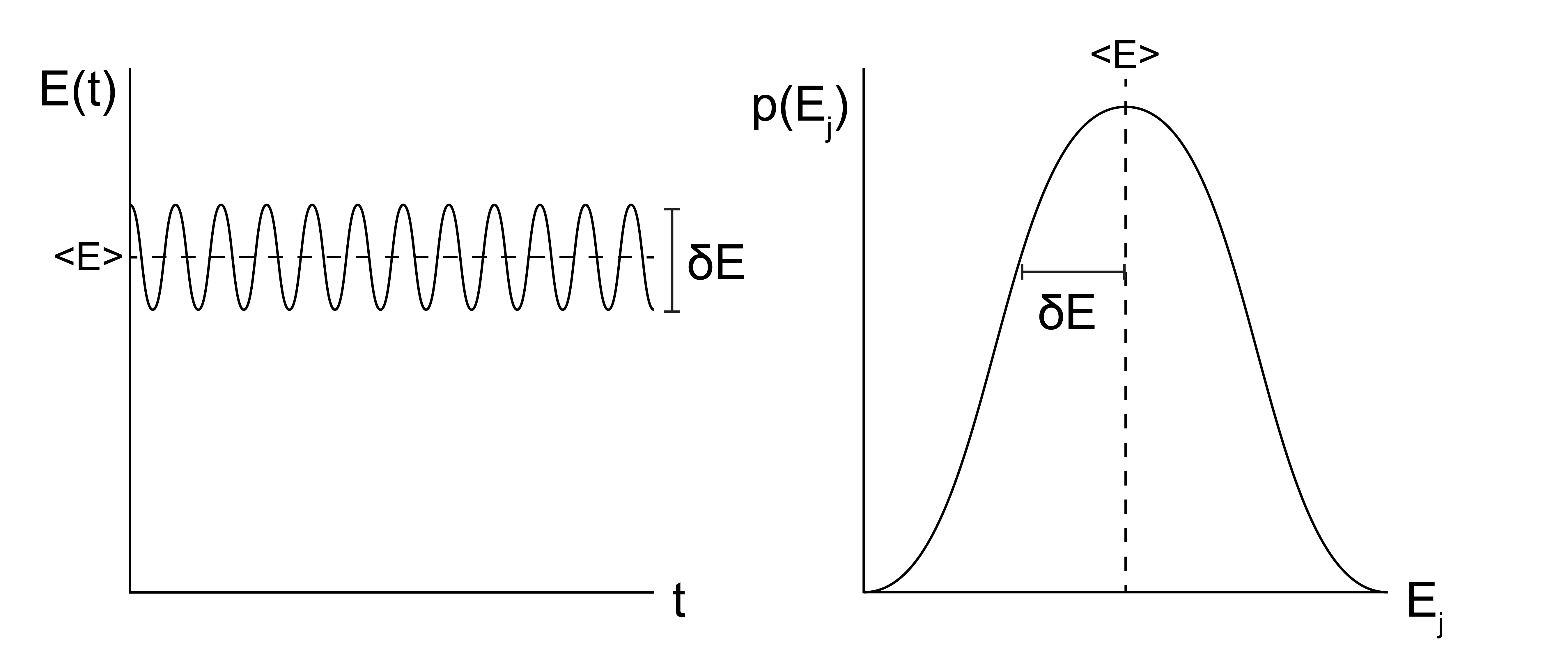
We begin by clarifying what is meant by fluctuations in this context. Consider the energy, \(E_j\), of a system described by the canonical ensemble (fixed \(NVT\)). The energy can vary between many different equivalent microstates of the canonical ensemble with different values of the energy \(E_j\), and we can define an ensemble average value of \(\langle E \rangle = \sum_j p_j E_j\). We can think of fluctuations in the energy in two different ways. First, we can imagine examining the system as a function of time, and periodically recording the instantaneous energy, \(E(t)\). At each snapshot of the system, \(E(t) = E_j\), in other words, the system by definition will be in some microstate such that its energy at time \(t\) will have a value equal to \(E_j\).

Recall the the ergodic hypothesis, that says that over sufficiently long times \(\int E(t) dt = \langle E \rangle\). That is, all microstates will be visited according to their Boltzmann-weighted probabilities and we can observe the ensemble average value of \(E\). Fluctuations by this definition then refer to the expected temporal variation in \(E(t)\) as the system evolves in time. However, because ergodicity establishes the equivalence of temporal measurements and ensemble averages, we can also think of fluctuations in the energy as a measure of the variance in the energy in the ensemble of microstates - i.e. simply a statistical quantity which reflects the distribution of energies accessible to a system. The key point here is that temporal fluctuations in the quantity are exactly equal to the statistical fluctuations in that quantity over long enough observation times such that ergodicity establishes the equivalence of the temporal average and ensemble average.

Having established the definition of fluctuations, why do we care? Well, our fluctuations are related to our

heat capacity

rate at which energy changes in a system due to a change in temperature

Prove that our ensemble-average variance, \(\langle ( \delta E)^2 \rangle \propto C_v\)

Hints

\(C_v = \left ( \frac{\partial \langle E \rangle}{\partial T} \right )_{N, V}\)

Show derivation

Taking the statistical definition of fluctuations, we can write the ensemble-average variance, \(\langle ( \delta E)^2 \rangle\), in the canonical ensemble as:

\[\begin{split}\begin{aligned} \langle ( \delta E)^2 \rangle &= \langle (E - \langle E \rangle )^2 \rangle \\ &= \langle E^2 - 2 E \langle E \rangle + \langle E \rangle^2 \rangle \\ &= \langle E^2 \rangle - 2 \langle E \rangle \langle E \rangle + \langle E \rangle ^2 \\ &= \langle E^2 \rangle - \langle E \rangle ^2 \end{aligned}\end{split}\]

Here we have simply rewritten the ensemble-averaged square fluctuation (i.e., the ensemble-averaged variance) in terms of ensemble averages of the energy itself. We can now use the equations from the canonical ensemble.

\[\begin{split}\begin{aligned} \langle ( \delta E)^2 \rangle = \langle E^2 \rangle - \langle E \rangle ^2 &= \sum_j p_j E_j ^2 - \left (\sum_j p_j E_j \right)^2 \\ &= \frac{1}{Z}\sum_j E_j^2 e^{-\beta E_j} - \left ( \frac{1}{Z} \sum_j E_j e^{-\beta E_j}\right )^2 \end{aligned}\end{split}\]

We next recognize that from the definition of the canonical partition function, \(Z = \sum_j e^{-\beta E_j}\), we get \(\frac{\partial Z}{\partial \beta} = -\sum_j E_j e^{-\beta E_j}\). Therefore the above expression becomes:

\[\begin{split}\begin{aligned} \langle ( \delta E)^2 \rangle &= \frac{1}{Z} \left ( \frac{\partial^2 Z}{\partial \beta^2} \right )_{N, V} - \left ( \frac{1}{Z} \left ( \frac{\partial Z}{\partial \beta} \right )_{N, V} \right )^2 \\ &= \frac{\partial}{\partial \beta} \left ( \frac{1}{Z} \frac{\partial Z}{\partial \beta} \right )_{N, V} \\ &= \frac{\partial}{\partial \beta} \left ( \frac{\partial \ln Z}{\partial \beta} \right )_{N, V} \end{aligned}\end{split}\]

Note the use of the product rule to simplify the first line to the second line. We recall from Lecture 3 that \(\langle E \rangle = -\left ( \frac{\partial \ln Z}{\partial \beta} \right )_{N, V}\) to get:

\[\begin{split} \langle ( \delta E)^2 \rangle &= -\left ( \frac{\partial \langle E \rangle}{\partial \beta} \right )_{N, V} \\ &= k_B \left ( \frac{\partial \langle E \rangle}{\partial T} \right )_{N, V} \left ( \frac{\partial T}{\partial T^{-1}} \right )_{N, V}\\ &= k_B T^2 \left ( \frac{\partial \langle E \rangle}{\partial T} \right )_{N, V} \\ &= k_BT ^2 C_V \end{split}\]

In the last line, we recognize that \(\left ( \frac{\partial \langle E \rangle}{\partial T} \right )_{N, V}\) is the heat capacity at constant volume, an experimentally measurable material constant.

This relationship is remarkable - it shows that the fluctuation (either with respect to time or with respect to the variation in the statistical ensemble) of energy in a system at fixed \(NVT\) is related to the rate at which energy in that system changes due to changes in the temperature. We call \(C_V\) a thermodynamic response function; that is, it shows the response of a system (i.e. change in energy) at equilibrium to a change in a parameter (i.e. the temperature). The relation above shows that microscopic fluctuations in the energy are a measure of the thermodynamic response of a system.

This relationship is strictly derived only at equilibrium, since everything we have done so far in statistical mechanics is at equilibrium; it turns out that similar relationships between statistical fluctuations and the response of a system also occur in non-equilibrium processes, leading to the so-called fluctuation-dissipation relationship, but that is outside of the scope of this lecture.

The relationship between fluctuations and a thermodynamic response illustrates a new means of calculating the heat capacity of the material. Without knowledge of this relationship, the simplest way to calculate the heat capacity would be to perform multiple experiments at different temperatures, measure the corresponding system energy, and equate \(C_V\) to the slope of the resulting line. Instead, our equation for heat capacity shows that we could take a single system at a fixed temperature and instead measure the fluctuations of the energy over time to obtain \(C_V\) in a single experiment. Such measurements will be possible using computer simulations as we will discuss in future lectures. We could also derive the fluctuations of other quantities, such as the density, and connect these to other materials parameters as a general means of computing response functions from equilibrium fluctuations.

Size of fluctuations and the equivalence of ensembles

The next question we will address how large fluctuations actually are relative to the average energy of the system. If fluctuations are much smaller than the average energy of the system, then the system energy will appear approximately constant. To determine the relative size of fluctuations, we recognize that the heat capacity, \(C_V\), is extensive and scales with the number of particles of the system, and thus is of order \(N\) (this was explicitly shown for an ideal gas). The energy, \(E\), is also extensive and scales with \(N\) (also shown for an ideal gas). The ratio of fluctuations to the average energy is then:

\[\begin{split}\begin{aligned} \frac{\sqrt{\langle ( \delta E)^2 \rangle}}{\langle E \rangle} &= \frac{\sqrt{k_BT ^2 C_V}}{\langle E \rangle} \\ &\approx \frac{\sqrt{N}}{N}\\ &\approx N^{-1/2} \end{aligned}\end{split}\]

This scaling analysis indicates that if \(N\) is a large number (e.g. on the order of \(10^{23}\) particles), then the ratio of fluctuations to the average energy approaches zero and the energy of the system is effectively constant. Thus, in the large \(N\) limit the average energy calculated from the canonical ensemble will be identical to the average energy of a microcanonical ensemble because energy fluctuations are negligible - and this is exactly the limit in which classical thermodynamics is valid.

To illustrate this point in just a bit more detail, we can write the equation for the canonical partition function by summing over all energy levels, and including the explicit degeneracy of energy level \(\nu\):

\[Z(N,V,T) = \sum_\nu \Omega(N,V,E_\nu) e^{-\beta E_\nu}\]

In the large \(N\) limit, we just showed that only a single value of \(E_\nu\), the ensemble average value, is meaningful, as fluctuations away from this value are unlikely. Thus, the degeneracy \(\Omega(N,V,\langle E \rangle)\) is significantly larger than any other term in the summation, and we can write the partition function instead as:

\[Z(N,V,T) = \Omega(N,V,\langle E \rangle) e^{-\beta\langle E \rangle}\]

Taking the logarithm of this expression and equating to the Helmholtz free energy yields:

\[\begin{split}\begin{aligned} F &= -k_BT \ln Z(N,V,T) \\ &= -k_B T \ln \left [ \Omega(N,V,\langle E \rangle) e^{-\beta\langle E \rangle} \right ] \\ &= \langle E \rangle -k_B T \ln \Omega(N,V,\langle E \rangle) \end{aligned}\end{split}\]

We can compare this last expression to the thermodynamic definition of the Helmholtz free energy, \(F = E - TS\). Therefore, we get that \(S = k_B \ln \Omega(N,V,\langle E \rangle)\), the Boltzmann entropy used to define the microcanonical ensemble, and we see that the two ensembles make equivalent predictions for the Helmholtz free energy. Similar measures of equivalency could be performed in the thermodynamic limit for other ensembles as well.

There are thus four important conclusions to draw from our study of fluctuations:

1. that in the thermodynamic limit, fluctuations are negligible, and hence we can discuss single values of thermodynamic variables as being equivalent to ensemble averages;

2. that in the thermodynamic limit all ensembles are equivalent, and hence we can use any ensemble that is mathematically convenient to relate molecular properties to macroscopic observables;

3. that microscopic fluctuations are proportional to a response function, both in equilibrium and in non-equilibrium processes;

4. fluctuations are measurable properties of a system that can be used to inform experimental measurements (e.g. in light scattering).

Summary of other topics

We have now finished our overview of statistical mechanics and will transition into an alternative approach to calculating the statistical properties of many-body, interacting systems via computer simulations. However, it is useful to emphasize that we have only scratched the surface of modern statistical mechanics, and that there many other topics of importance. Briefly, here are some topics of interest that we have not discussed:

• Kinetic theory of gases (although we will touch on this in the next unit)

• Topics in non-equilibrium statistical mechanics, such as linear response theory

• Renormalization group approaches to phase transitions

• Correlation functions and order parameters

• Landau-Ginsburg models for phase transitions

• Statistical mechanics of surfaces

If you’re interested in these topics, I am happy to point you toward relevant textbooks.

Link to Shared Notes