Temperature and velocities in MD

Additional Readings for the Enthusiast

• Frenkel and Smit [2], Ch. 6.1

Goals for Today’s Lecture

• Use the Maxwell-Boltzmann distribution to compute initial particle velocities in simulation

• Relate ensemble-average velocities to ensemble-average temperature

• Describe the concept of a simulation thermostat, including the Andersen thermostat

Sampling the canonical ensemble in MD simulations

We have now discussed the basic equations of motion for a MD simulation, but have not clearly connected to a statistical ensemble. In Monte Carlo simulations, the statistical ensemble sampled (i.e., the canonical ensemble) is enforced by choosing configurations with a probability proportional to the Boltzmann factor.

What statistical ensemble is “default” for basic MD simulations?

Click for answer

In MD simulations, the statistical ensemble is enforced by the equations of motion. For basic MD, we integrate Newton’s equations of motion, which are conservative, so the total energy of the system (kinetic + potential energy) is fixed. As a result, the MD algorithm described in above samples the microcanonical ensemble. This ensemble is perfectly fine for some systems, such as isolated molecules in the gas phase that are not in contact with a heat bath.

In many problems of interest we would rather model a system that is at a constant temperature and samples the canonical ensemble since this is more representative of most physical systems. We thus need to modify our equations of motion to add a constraint that maintains a constant temperature instead of constant energy.

We will now seek to derive an algorithm for constant temperature MD simulations via the implementation of a simulation thermostat. First, however, there is a more fundamental question - how do we define temperature in a molecular dynamics simulation? Answering this question will also tie up a loose end from the previous class, namely how we should initialize the velocities of particles in our system.

Maxwell-Boltzmann distribution

So far in this class, we have dealt solely with potential energy functions that are a function of particle positions. However, in a classical simulation, a particle configuration is specified by particle momenta (i.e., velocities, denoted \(\textbf{v}^N\)) in addition to particle positions (denoted \(\textbf{r}^N\)).

The complete energy of the system is then given by both the potential energy, \(P(\textbf{r}^N)\), and the kinetic energy, given by \(K(\textbf{v}^N)\). Note an important feature - in general for a conservative Newtonian system, the potential energy is only a function of particle positions, while the kinetic energy is only a function of particle velocities/momenta. The two contributions are thus separable - i.e., their contributions to the partition function can be factorized.

Let’s then consider the distribution of molecular velocities associated with the kinetic energy, \(K(\textbf{v}^N)\), since this term in the total energy is independent of the potential energy term. We can write the kinetic energy of particle \(i\) as:

\[\begin{aligned} K(\textbf{v}_i) = \frac{1}{2}m\textbf{v}_i \cdot \textbf{v}_i = \frac{1}{2}mv^2 \end{aligned}\]

Here, the speed \(v\) is the magnitude of the velocity vector, \(\textbf{v}_i\). Now, we ask the probability that a particle obtains a particular velocity vector near the point where \(\textbf{v}_i = (v_x, v_y, v_z)\).

Since we are in the classical limit and treat particle coordinates/velocities as a continuum, we no longer ask the probability of one specific velocity vector, but rather the probability of finding a velocity within a small range of velocities. That is, if we think of the space of possible velocities as a 3D volume with axes \(v_x, v_y,\) and \(v_z\), then we want to calculate the probability of finding a particle with a velocity within an infinitesimal volume \(dv_x dv_y dv_z\) centered on \(v_x, v_y, v_z\) in this velocity space. We can write this probability density (i.e. probability per unit volume) in the canonical ensemble as:

\[\begin{split}\begin{aligned} \rho(v_x, v_y, v_z) &=\frac{e^{-\beta K(\textbf{v}_i)}}{Z} \\ &= \frac{1}{Z} \exp\left [ - \frac{m(v_x^2 + v_y^2 + v_z^2)}{2k_BT }\right ] \end{aligned}\end{split}\]

Here, \(Z\) is a partition function we calculate by enforcing that the probability of obtaining a velocity vector in the entire volume of the velocity space has to be 1:

\[\int_{-\infty}^{\infty} \int_{-\infty}^{\infty} \int_{-\infty}^{\infty} \frac{1}{Z}\exp\left [ - \frac{m(v_x^2 + v_y^2 + v_z^2)}{2k_BT }\right ] dv_x dv_y dv_z = 1\]

Show that \(Z = \left(\frac{m}{2\pi k_B T} \right)^{-3/2}\)

Show derivation

Using \(\int_{-\infty}^{\infty}\exp\left [-ax^2\right] = \sqrt{\frac{\pi}{a}}\):

\[\begin{split}\begin{aligned} Z &= \int_{-\infty}^{\infty} \int_{-\infty}^{\infty} \int_{-\infty}^{\infty} \exp\left [ - \frac{m(v_x^2 + v_y^2 + v_z^2)}{2k_BT }\right ] dv_x dv_y dv_z\\ &= \int_{-\infty}^{\infty}\exp\left [ - \frac{m(v_x^2)}{2k_BT }\right ] dv_x\int_{-\infty}^{\infty} \exp\left [ - \frac{m(v_y^2)}{2k_BT }\right ] dv_y\int_{-\infty}^{\infty} \exp\left [ - \frac{m(v_z^2)}{2k_BT }\right ] dv_z\\ &= \left(\frac{2\pi k_BT }{m}\right)^{3/2} \end{aligned} \end{split}\]

Our probability density for velocities is then the

Maxwell-Boltzmann distribution for velocities

\[\rho(v_x, v_y, v_z) = \left(\frac{m}{2\pi k_B T} \right)^{3/2} \exp\left [ - \frac{m(v_x^2 + v_y^2 + v_z^2)}{2k_BT }\right ]\]

This expression tells us that the probability of finding a particle with a velocity within an infinitesimal volume element \((dv_x, dv_y, dv_z)\) centered on the vector \(\textbf{v}_i = (v_x, v_y, v_z)\) is given by:

\[p(v_x, v_y, v_z) = \rho(v_x, v_y, v_z) dv_x dv_y dv_z\]

Integrating this expression over a finite volume of interest (in velocity space) yields the probability of finding a velocity within that volume. Recall that it is \(p\) that is normalized to be 1 across the entire space, not \(\rho\).

There are a few things to note about this distribution. First, each of component of the velocity vector is independent; that is, we can write:

\[\rho(v_x, v_y, v_z) = \rho(v_x) \rho(v_y) \rho(v_z)\]

and

\[\begin{split}\begin{aligned} \rho(v_x) &= \rho(v_y) = \rho(v_z) \\ &= \left(\frac{m}{2\pi k_B T} \right)^{1/2} \exp\left [ - \frac{mv_x^2}{2k_BT }\right ] \end{aligned}\end{split}\]

Second, the Maxwell-Boltzmann distribution is strictly only valid at equilibrium, because we use the canonical partition function in the derivation. However, that’s the only major assumption we make, other than that classical mechanics is valid (i.e. we are not moving at relativistic speeds and there are no strong quantum effects).

The Maxwell-Boltzmann distribution as a Gaussian distribution

If we look at the form of this distribution, we see that it follows a Gaussian (normal) distribution. Recall that a Gaussian function generally has the form:

\[f(x) = \frac{1}{\sigma \sqrt{2\pi}}\exp \left [-\frac{1}{2}\left (\frac{x-\mu}{\sigma}\right )^2 \right ]\]

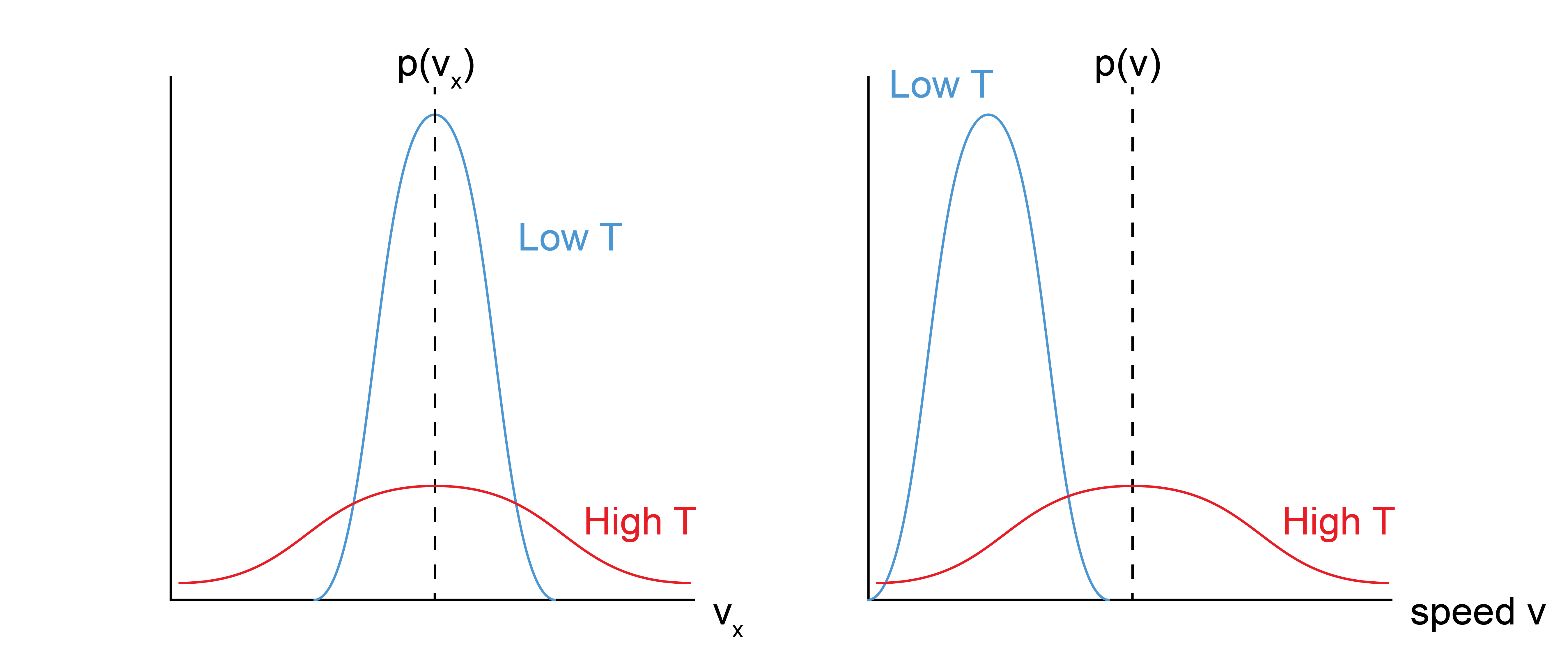
where \(\sigma^2\) is the variance and \(\mu\) is the mean. Comparing this form with the Maxwell-Boltzmann distribution for a single component of the velocity vector shows that the variance of the distribution is \(\sigma^2 = \frac{k_B T}{m}\) and the mean is \(\mu=0\). These two quantities tell us that as we increase the temperature of the system, the mean velocity is always zero, but we are increasingly likely to sample larger velocities.

In principle, we want to generate velocities such that the system begins at a particular, well-defined temperature. The Maxwell-Boltzmann distribution then tells us how to do this. Specifically, for each particle, we can generate three random numbers drawn from the Maxwell-Boltzmann velocity distribution at the desired temperature \(T\) to represent each of the three velocity components; again this is possible because each component is statistically independent.

In practice, it is worth noting that a property of Gaussian functions is that if \(X\) is normally distributed with a mean \(\mu\) and variance \(\sigma^2\), then \(Y=aX\) is also normally distributed with mean \(a\mu\) and variance \(a^2\sigma^2\). Thus, we only need a function that generates random numbers drawn from a Gaussian distribution with a mean of 0 and a variance of any number, and we can convert the results of that distribution to our chosen Maxwell-Boltzmann distribution by multiplying by an appropriate value of \(a\). Matlab has a built-in function to do this, for example.

Features of the Maxwell-Boltzmann distribution

First, we can calculate the distribution of speeds as opposed to velocities - that is, the distribution of \(v = \sqrt{\textbf{v}\cdot \textbf{v}}\). This requires an integral in spherical coordinates to represent all possible vector directions with a final result of:

\[\rho(v) = \left(\frac{m}{2\pi k_B T} \right)^{3/2} 4\pi v^2 \exp\left [ - \frac{mv^2}{2k_BT }\right ]\]

Again, recall that this is the probability density (per unit speed, since we multiply by \(dv\) to get the actual probability) of finding the particle with a speed near \(v\), but here \(v\) is always positive and is a scalar quantity. Unlike the velocity distribution, the mean of the speed distribution is non-zero, and instead we can show that:

\[\begin{split}\begin{aligned} \langle v \rangle &= \int_0^\infty v \rho(v) dv = \sqrt{\frac{8k_BT}{\pi m}}\\ \langle v^2 \rangle &= \int_0^\infty v^2 \rho(v) dv = \frac{3k_BT}{m} \end{aligned}\end{split}\]

This means that at higher temperatures the distribution of speeds broadens and shifts to higher values, indicating that particles move faster at higher temperatures, as expected.

So note the results we have so far: by assuming a set of particles that have velocities consistent with the canonical ensemble, we can relate the ensemble-average value of the speed squared to the temperature. Relating this last expression to the kinetic energy (for a set of all \(N\) particles) gives:

\[\begin{split}\begin{aligned} \langle K(\textbf{v}^N) \rangle &= \left \langle \frac{1}{2}Nmv^2 \right \rangle \\ &= \frac{1}{2}Nm \langle v^2 \rangle \\ &= \frac{3}{2}Nk_BT \end{aligned}\end{split}\]

This result, that the contribution of each particle to the ensemble-average kinetic energy is given by \(3/2 k_BT\), is exactly the result obtained from the equipartition theorem - each degree of freedom for the velocity, which is squared in the expression for the kinetic energy, contributes \(1/2 k_BT\) to the corresponding ensemble-average energy (kinetic energy in this case).

Say I am simulating the liquid and vapor phases of a system near the phase boundary (i.e., at the same temperature, where both phases are stable). Which system’s particles have a higher velocity?

Click for answer

Because the two systems are at the same temperature, the distribution of their molecular velocities are the same, even though we may conventionally think that gas molecules move “faster” than liquid molecules. In reality, it’s that liquid-phase molecules collide more frequently so that their velocity vectors change more rapidly, but the distribution of velocities remains the same as a corresponding vapor-phase system. Of course, typically we also associate gases with higher temperature phases, in which case our results do indeed show that their molecular speeds would be faster on average.

Calculating temperature in a molecular simulation

With the Maxwell-Boltzmann relationship in hand, we can now see a method to calculate the temperature in a molecular simulation. Specifically, we have the relation:

\[\begin{aligned} \frac{1}{2}Nm \langle v^2 \rangle &= \frac{3}{2}Nk_BT \end{aligned}\]

This expression gives us an operational definition of the temperature; while strictly we only relate the ensemble-average kinetic energy to the temperature, we can approximate the temperature as a function of time by:

\[\begin{aligned} T(t) = \frac{1}{N} \sum_i^N \frac{m_i v_i(t)^2}{3k_B} \end{aligned}\]

Using this definition, the temperature will fluctuate for a system at constant energy (i.e. using standard MD algorithms) and also for a system at “constant” temperature (i.e. using a thermostat as described below) since the relationship between temperature and kinetic energy is only valid in ergodic systems. Thus, if a simulation is run for long enough at constant temperature such that the Maxwell-Boltzmann distribution correctly describes particle speeds, then this relationship should generate the expected ensemble-average temperature. Note that the instantaneous temperature is still not rigorously defined - we would say that the temperature of the system is the ensemble-average temperature, and the instantaneous temperature is defined only to facilitate calculations (i.e. to maintain temperature via the thermostat described below).

Andersen thermostat

We have now derived the Maxwell-Boltzmann distribution for particle velocities in the canonical ensemble, and showed that we could link the ensemble-average temperature to the ensemble-average kinetic energy as a means of defining the simulation temperature. However, we have yet to discuss how to actually maintain a well-defined simulation temperature so that our system samples the canonical ensemble. We will now discuss this by defining a simulation

thermostat

in simulation, an algorithm to conserve the system temperature

First, you may immediately realize that if \(T(t) = \sum_i^N \frac{m_i v_i(t)^2}{3k_B N}\), then we can enforce a constant temperature by just rescaling the velocities every time step. Velocity rescaling in principle is fine since it does not affect the relative positions of particles, and hence will not result in unphysical states (e.g. particles overlapping).

What problems could you see with velocity scaling to maintain constant temperature?

Click for answer

The problem with this approach is that it would eliminate fluctuations in the kinetic energy and may not capture the correct Maxwell-Boltzmann distribution of particle velocities expected in the canonical ensemble.

Instead, we will describe an approach called the

Andersen thermostat

A simulation thermostat which keeps constant temperature by assuming that particles stochastically collide with some particle in the external heat reservoir.

In between these collisions, the system evolves at constant total energy; each collision essentially ensures that the system samples different possible constant system energies (i.e. different microcanonical ensembles) with the correct Boltzmann weight.

An Andersen thermostat is implemented by selecting a set of particles (or a single particle) stochastically with a frequency given by a coupling parameter, \(\eta\), and resetting their velocities according to the Maxwell-Boltzmann distribution; this represents a collision with a particle in the thermal reservoir. Assuming that collisions are uncorrelated, the probability with which each particle collides with the bath at each timestep is given by:

\[p(\Delta t; \eta) = \eta \Delta t\]

This expression is based on the mean number of collisions expected during an interval \(\Delta t\). The collision frequency, \(\eta\), is usually specified in terms of the timestep. It can be shown that this procedure correctly reproduces properties of a canonical ensemble since the kinetic energy will sample the correct distribution and the temperature is only a function of the particle velocities. For example, the Andersen thermostat will produce the correct Maxwell-Boltzmann distribution of velocities and can exactly reproduce Monte Carlo simulations that sample the canonical ensemble. The coupling parameter can be tuned and there is not necessarily an optimal value; typical values are on the order of \(\eta = \frac{0.01}{\Delta t}\) to \(\eta = \frac{0.001}{\Delta t}\) so that velocities are not reset too frequently, which could interfere with measurements of dynamical behaviors (i.e., the measurement of the diffusion coefficient).

Note that the Andersen thermostat changes the velocities of particles at time \(t\), and hence requires an equation of motion in which velocities are specified, such as the Velocity Verlet algorithm. An example algorithm for a MD simulation using the Andersen thermostat then consists of the following steps:

1. Choose a starting configuration, \(\mathbf{r}^N(t=0)\).

2. Generate initial particle velocities, \(\textbf{v}^N(t=0)\), by sampling from the Maxwell-Boltzmann velocity distribution at a given temperature \(T\).

3. Compute the forces acting on all particles, \(\textbf{f}^N(t)\).

4. Update the positions to time \(\textbf{r}^N(t+\Delta t)\).

5. Update the velocities to \(\textbf{v}^N(t+1/2\Delta t)\) according to the Velocity-Verlet algorithm.

6. Calculate the new forces \(\textbf{f}^N(t+\Delta t)\).

7. Finish the velocity update to \(\textbf{v}^N(t+\Delta t)\)

8. Iterate over all particles and stochastically attempt to select a particle with probability \(\eta \Delta t\); if selected, reset the particle velocity vector by sampling each component from the Maxwell-Boltzmann velocity distribution.

9. Repeat steps 3-8 until a sufficient number of timesteps have elapsed. Periodically compute and save the value of some observables (e.g., temperature, pressure).

10. Approximate the ensemble-average value of the saved observables by averaging over states sampled during a period of time during which the system is at equilibrium.

Note again that this algorithm now introduces a stochastic element to molecular dynamics, unlike the basic MD algorithm which in principle is deterministic. Finally, it is important to recognize that the Andersen thermostat is just one simple approach for maintaining the system temprature, and is no longer commonly used in practice in favor of more advanced techniques (e.g. the Nose-Hoover thermostat) that are considered more reliable.

Link to Shared Notes