Application of independent subsystems: the Langmuir isotherm

Additional Readings for the Enthusiast

• YouTube Introduction

Goals for today’s lecture

• Derive the fraction of absorbed sites on a surface solely based on the pressure of the surrounding gas and the binding energy.

The Langmuir Isotherm

The previous lecture shows that statistical mechanics can reproduce classical thermodynamic relationships from first-principles. We will now test a second example of the three-step approach for studying independent particles by deriving the Langmuir adsorption isotherm.

Consider a system of \(N\) ideal gas particles that can adsorb onto a surface. Physically, this system could represent the adsorption of reactants onto a catalytic surface. We define the number of adsorbed particles as \(N_a\) and the remaining number of free gas particles as \(N-N_a\). Particles adsorb favorably with an energy of \(-\epsilon_a\) per particle.

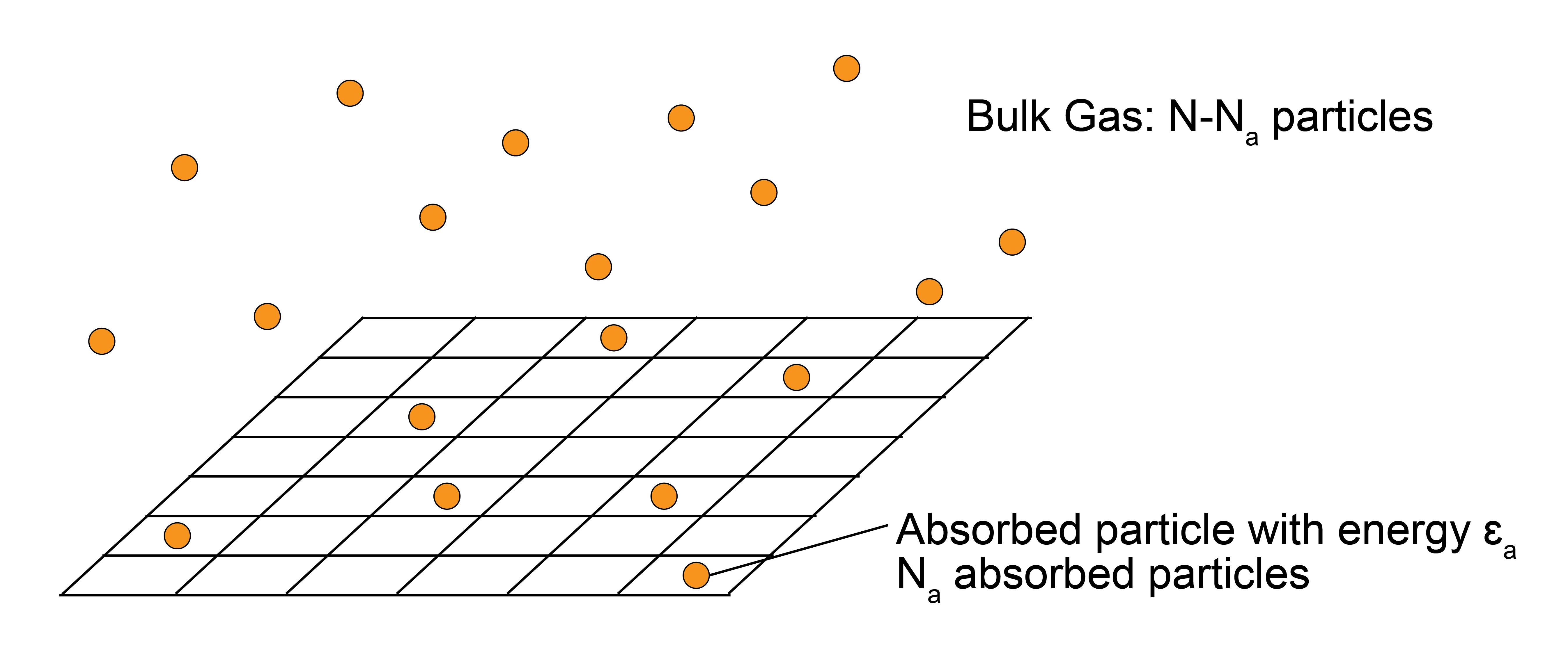
To simplify our treatment, we assume all particles adsorb onto a lattice of discrete with \(N_s\) possible binding sites, of which \(N_a\) are occupied assuming that only a single particle can bind to each site (with \(N_s > N_a\), allowing for all particles to adsorb). All binding sites are assumed to be independent; that is, the arrangement of particles does not affect the energy of the system. The quantity we will determine is the fraction of the surface that is occupied as a function of the pressure of the surrounding gas, \(f_a(P)\).

We next have to consider what ensemble to use to solve this problem. We can think of particles adsorbed to the surface and particles free in the bulk as two distinct sets of particles such that particles are free to exchange between the surface and bulk. The number of particles adsorbed to the surface, \(N_a\), is thus allowed to vary. \(\langle N_A \rangle\) will be determined at equilibrium which is reached when each particle adsorbed to the surface has a constant chemical potential, \(\mu_a\), that is equal to the chemical potential of each particle in the bulk, \(\mu_b\).

Which ensemble is most appropriate here? We are treating the surface as the system.

Microcanonical ensemble

Incorrect, as the number of particles in our system can change, and our energy can change. Try again

Canonical ensemble

Incorrect, as the number of particles in our system can change. Try again

Grand canonical Ensemble

Since the number of particles can vary on the surface, the natural ensemble to consider is the grand canonical ensemble because the natural variables of the ensemble, $\mu V T$, are the same variables that are constant at equilibrium.

Isothermal-isobaric ensemble

Incorrect, as the number of particles in our system can change and our pressure can change. Try again

The surface has \(N_s\) potential binding sites; each binding site is either occupied or not, with the number of occupied sites (\(N_a\)) fluctuating. We aim to find an expression for \(f_a = \frac{N_a}{N_s}\). Since \(N_a\) can vary, we really seek the ensemble average value of \(N_a\), so that \(f_a = \frac{\langle N_a \rangle}{N_s}\).

Since each binding site is independent and identical, we can factorize the partition function by treating each site as a subsystem that is either occupied or unoccupied, meaning that a single particle is adsorbed to the site or not. Since the sites are spatially distinct, each subsystem is distinguishable. We then write the grand canonical ensemble partition function for the whole surface as:

\[\Xi_s = \xi_s^{N_s}\]

where \(\xi_s\) is the single-site grand canonical partition function given as:

\[\begin{aligned} \xi_s = \sum_{j}e^{-E_j \beta}e^{\mu_a N_j \beta} \end{aligned}\]

Why are we working with the distinguishable subsystem equation?

Click for answer

Here we are working from the viewpoint of the sites not the particles. The sites are distinguishable, whereas the particles are not.

Show that \(\Xi_s = \left ( 1 + e^{\epsilon_a \beta}e^{\mu_a \beta} \right )^{N_s}\).

Show derivation

For a single site, there are only two possible values of \(N_j\): either the site is occupied, for which \(N_j = 1\), or the site is unoccupied, for which \(N_j = 0\). Similarly, there are only two possible energies: if \(N_j = 1\), \(E_j = -\epsilon_a\), and if \(N_j = 0\), \(E_j = 0\). Therefore the single-site partition function is:

\[\begin{split}\begin{aligned} \xi_s &= e^{0 \beta}e^{0 \beta} + e^{-\epsilon_a \beta}e^{\mu_a \beta} \\ &= 1 + e^{\epsilon_a \beta}e^{\mu_a \beta} \\ \Xi_s &= \xi_s^{N_s}\\ &= \left ( 1 + e^{\epsilon_a \beta}e^{\mu_a \beta} \right )^{N_s} \end{aligned}\end{split}\]

Next, we write an expression for the grand potential:

\[\begin{split}\begin{aligned} \Sigma_G &= - k_B T \ln \Xi_s \\ &= - N_s k_B T \ln \left ( 1 + e^{\epsilon_a \beta}e^{\mu_a \beta} \right ) \end{aligned}\end{split}\]

Show that \(f_a = \frac{ e^{\epsilon_a \beta}e^{\mu_a \beta}}{ 1 + e^{\epsilon_a \beta}e^{\mu_a \beta}}\).

Show derivation

We need to relate this thermodynamic potential to the quantity of interest, \(\langle N_a \rangle\). Recall that we can write an expression for \(\Sigma_G\), which is a function of the natural variables \(\mu_a V T\), as:

\[\begin{split}\begin{aligned} \Sigma_G (\mu_a, V, T) &= E(N, V, S) - TS - \mu_a N_a \\ d\Sigma_G &= dE - TdS - SdT - \mu_a d N_a - N_a d \mu_a \\ &= TdS - PdV + \mu_a dN_a - TdS - SdT - \mu_a d N_a - N_a d \mu_a \\ &= -S dT - PdV - N_a d \mu_a \end{aligned}\end{split}\]

Therefore, we recognize that \(\left ( \frac{\partial \Sigma_G}{\partial \mu_a} \right )_{V,T} = - N_a\), so:

\[\begin{split}\begin{aligned} N_a &= -\left ( \frac{\partial \Sigma_G}{\partial \mu_a} \right )_{V,T} \\ &= \frac{ N_s e^{\epsilon_a \beta}e^{\mu_a \beta}}{ 1 + e^{\epsilon_a \beta}e^{\mu_a \beta} }\\ f_a &= \frac{ N_a }{N_s} \\ &= \frac{ e^{\epsilon_a \beta}e^{\mu_a \beta}}{ 1 + e^{\epsilon_a \beta}e^{\mu_a \beta}} \end{aligned}\end{split}\]

We now have an expression in terms of the chemical potential of the particles adsorbed to the bulk, but we’d like an expression in terms of the pressure of the bulk gas. At equilibrium, we know that \(\mu_a = \mu_b\), so we can calculate the chemical potential for particles in the bulk and relate this to the pressure. Since the gas molecules are ideal, non-interacting particles, these particles are described as an ideal gas. As a result, we can substitute in the expression for the chemical potential derived from the ideal gas (canonical) partition function in our previous lecture and use this for the chemical potential of particles in the bulk:

\[\begin{split}\begin{aligned} \mu_b &= -k_B T \ln \left( \frac{2\pi m k_BT}{h^2}\right )^{3/2} + k_B T \ln \frac{N-N_a}{V} \\ &= -k_B T \ln \left [ \frac{V}{(N-N_a)\lambda^3}\right ] \end{aligned}\end{split}\]

Note that we use \(\lambda\) (the thermal de Broglie wavelength) to simplify the notation. We use the ideal gas equation of state (\(V = \frac{(N-N_a) k_B T}{P}\)) to obtain a pressure dependence:

\[\begin{split}\begin{aligned} \mu_b &= -k_B T \ln \left [ \frac{(N-N_a)k_B T}{P(N-N_a)\lambda^3}\right ] \\ &= k_B T \ln \left ( \frac{P\lambda^3}{k_B T}\right ) \end{aligned}\end{split}\]

Finally, we now require the condition \(\mu_a = \mu_b\) to find an expression for \(f_a\). Substituting in the expression for \(\mu_b\) to our prior expression for \(f_a\) yields:

\[\begin{split}\begin{aligned} f_a &= \frac{ \left ( \frac{P\lambda^3}{k_BT}\right )e^{\epsilon_a \beta}}{1 + \left ( \frac{P\lambda^3}{k_BT}\right ) e^{\epsilon_a \beta}} \\ &= \frac{P / P_0}{1 + P / P_0} \end{aligned}\end{split}\]

Here, we define \(P_0 = \left ( \frac{k_B T}{\lambda^3}\right )e^{-\epsilon_a / k_BT}\) as a constant (equal to the pressure for which \(f_a = 0.5\)) that does not depend on \(f_a\) or on \(P\). This expression is our goal - we relate the pressure to the fraction of occupied sites, \(f_a\). We can rearrange this to equivalently write:

\[f_a = \frac{P}{P + P_0}\]

This last expression is referred to as the

Langmuir adsorption isotherm

\(f_a = \frac{P}{P + P_0}\); shows that as the pressure of the system increases, the surface coverage increases until eventually plateauing.

Similar isotherm behavior is observed in a number of experimental systems. Note also that by solving for the value \(P_0\), which is equivalent to the pressure where the surface is half-occupied, we can find a value for \(\epsilon_a\) or the binding energy if the thermal de Broglie wavelength is known. Thus, statistical mechanics provides a valuable connection between microscopic and macroscopic observables relevant to surface occupancy.

Link to Shared Notes