Non-ideal mixtures

Additional Readings for the Enthusiast

Tester and Modell [4], Ch. 9.8, 15.3

Goals for Today’s Lecture

• Define and derive Raoult’s Law for vapor-liquid equilibrium

• Read binary phase diagrams; define equilibrium compositions

• Describe how non-ideality causes deviations from Raoult’s Law; modify Raoult’s Law for non-ideal mixtures

• Plot and understand Gibb’s free energy of mixing (\(\Delta G_{mix}\)) in liquid mixtures

• From plots of \(\Delta G_{mix}\), identify when phase separation and mixing occurs

Raoult’s Law

In the last lecture, we defined two simplified approximations for mixtures: an ideal-gas mixture and an ideal solution. An ideal solution is a solution in which the intermolecular interactions between system constituents are sufficiently similar that the interactions between different components are equivalent to the interactions between pure components with themselves. An ideal-gas mixture further approximates all components as ideal gases. For these systems, we derived the Lewis-Randall rule for the fugacities as:

\[\begin{split}\begin{aligned} \hat{f}_i^\textrm{IS} &= x_i f_i \\ \hat{f}_i^\textrm{IG} &= y_i P \end{aligned}\end{split}\]

Where \(\hat{f}\) denotes the fugacity of a component in a mixture, and \(f_i\) is the single-phase fugacity.

We can use these expressions to derive an expression for phase equilibrium between a vapor phase and a liquid phase, in which we assume the vapor phase is an ideal-gas mixture and the liquid phase is an ideal solution. Phase equilibrium between these completely ideal phases thus represents an extreme of behavior and we will then consider deviations from ideality.

First, recall that the condition for phase equilibrium in multicomponent systems is:

\[\begin{aligned} \hat{f}_i^\textrm{vap} &= \hat{f}_i^\textrm{liq} \end{aligned}\]

This expression has to hold for each component of our mixture. Treating the vapor phase as an ideal-gas mixture and the liquid phase as an ideal solution gives:

\[\begin{split}\begin{aligned} \hat{f}_i^\textrm{IG} &= y_i P \\ \hat{f}_i^\textrm{IS} &= x_i f_i \\ \therefore x_i f_i^\textrm{liq} &= y_i P \end{aligned}\end{split}\]

We previously derived the Poynting correction as an approximation for the fugacity of a liquid-phase component, given by:

\[\begin{aligned} f_i^{\textrm{liq}} = f_i^{\textrm{sat}} \exp\left [ \frac{V_i^{\textrm{liq}}(P-P_i^{\textrm{sat}})}{RT} \right ] \end{aligned}\]

At vapor-liquid equilibrium, the fugacity of pure component \(i\) in the liquid phase is equal to the fugacity of pure component \(i\) in the vapor phase. Since the vapor phase of the mixture is an ideal-gas mixture, pure component \(i\) in the vapor phase is also an ideal gas. Therefore we have:

\[\begin{split}\begin{aligned} f_i^\textrm{sat} &= f_i^\textrm{vap, sat} = P_i^\textrm{sat} \\ f_i^{\textrm{liq}} &= P_i^\textrm{sat} \exp\left [ \frac{V_i^{\textrm{liq}}(P-P_i^{\textrm{sat}})}{RT} \right ] \end{aligned}\end{split}\]

Typically, the exponential term is negligible unless the pressure significantly varies from the saturation pressure, so we can approximate the fugacity of the ideal solution as:

\[\begin{aligned} f_i^\textrm{liq} &\approx P_i^\textrm{sat} \end{aligned}\]

The notation emphasizes that the fugacity of component \(i\) in the liquid phase is equal to the saturation pressure of that pure component. Combining with the condition of phase equilibrium leads to

Raoult’s Law

\[\begin{split}\begin{aligned} x_i f_i^\textrm{liq} &= y_i P \\ \therefore x_i P_i^\textrm{sat} &= y_i P \end{aligned}\end{split}\]

Raoult’s law states that the partial pressure of component \(i\) in the vapor phase (\(y_i P\)) at equilibrium with a liquid solution is related to the saturation pressure of pure component \(i\) weighted by its mole fraction in the liquid solution. Since mole fractions have to sum to 1, we can also then write:

\[\begin{aligned} \sum_i^n x_i P_i^{\textrm{sat}} = \sum_i^n y_i P = P \end{aligned}\]

Binary phase diagrams

We can plot the equilibrium conditions predicted by Raoult’s Law for a two-component system by drawing a binary phase diagram. In a binary phase diagram,

• the y-axis is typically the pressure (in which case the temperature is constant for the entire phase diagram)

• or temperature (in which case the pressure is held constant for the entire phase diagram)

• the x-axis represents composition in terms of mole fraction

Such diagrams are called P-x-y or T-x-y diagrams respectively, with the \(x\) and \(y\) referring to the fact that the composition axis can refer to both composition in vapor and liquid phases. Each phase diagram represents a slice through a higher-dimensional \(PVT\) space.

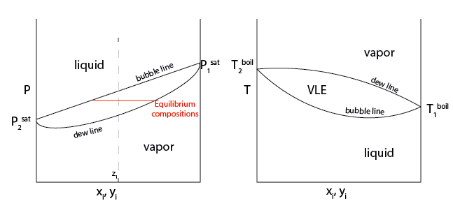
Consider an example P-x-y diagram for a system described well by Raoult’s Law. The overall mole fraction of the mixture is denoted as \(z_i\). At a high pressure, a single liquid phase is observed and \(x_i = z_i\) in this phase. At a low pressure, a single vapor phase is observed and \(y_i = z_i\) in this phase. For intermediate pressures, there is a region of the phase diagram in which we would observe

vapor-liquid equilibrium

also known as VLE. Region of phase space where vapor and liquid are both stable

If we were to imagine compressing an initially vapor system with composition \(z_i\) infinitely slowly, the pressure at which we first observe a drop of liquid is called the dew point, which corresponds to the first pressure for which the conditions of VLE are satisfied. Recall that these conditions are:

\[\begin{aligned} \hat{f}_i^\textrm{liq} &= \hat{f}_i^\textrm{vap} \end{aligned}\]

dew line

The locus of dew points for all possible system compositions, and represents the lower (on a P-x-y diagram) or upper (on a T-x-y diagram) bound of the phase envelope (or binodal) encapsulating the region of VLE.

Similarly, we could imagine expanding an initially liquid system until we first observe a vapor bubble, leading to the

bubble point

the pressure at which we first observe a vapor bubble

bubble line

the locus of all bubble points

What is the composition of each of the phases in the VLE phase envelope?

Click for answer

In the VLE phase envelope, the composition of the vapor phase at any given pressure and temperature is equal to the composition of the corresponding point on the dew line (i.e., at the same pressure and temperature) while the composition of the liquid phase is equal to the composition of the corresponding point on the bubble line. Equivalently, we can imagine drawing a horizontal line connecting the bubble and dew lines - called a tie line - and the intersections of the tie line with the bubble and dew lines defines the compositions of the phases present at equilibrium. Since these compositions are determined only by the temperature and pressure, the overall composition of the system (\(z_i\)) only changes the relative amounts of the two phases present in the system. This behavior is analogous to how the total volume of a single-component system at the saturation pressure changes only the relative amounts of the two phases present.

VLE for non-ideal systems

Raoult’s Law defines the simplest possible phase behavior in a binary system since we assume ideality for both phases. Raoult’s Law gives rise to a linear bubble line on P-x-y plots; this can be shown by applying the mass balance constraint to Raoult’s Law:

\[\begin{split}\begin{aligned} x_i P_i^\textrm{sat} &= y_i P \\ \sum_i y_i P &= P = \sum_i x_i P_i^\textrm{sat} \\ \therefore P &= x_1 P_1^\textrm{sat} + (1-x_1) P_2^\textrm{sat} \\ &= P_2^\textrm{sat} + x_1 (P_1^\textrm{sat} - P_2^\textrm{sat}) \end{aligned}\end{split}\]

Ideal behavior is thus easy to see from P-x-y plots, as deviations from ideality will give rise to non-linear bubble lines.

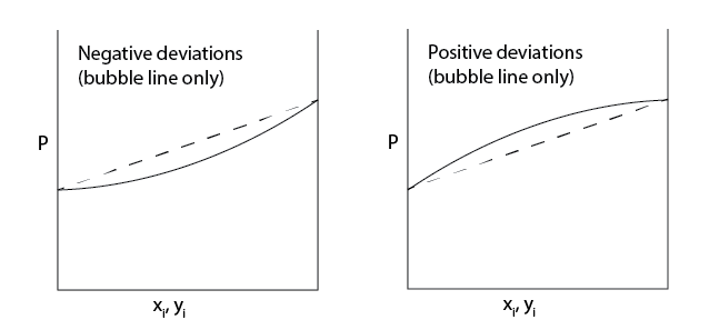
• Solutions that have pressures larger than expected from Raoult’s Law are said to exhibit positive deviations, so that \(P > \sum_i^n x_i P_i^{\textrm{sat}}\). Positive deviations indicate a shift in the equilibrium toward the vapor phase (i.e., the fugacities of components in the liquid phase are higher than expected of an ideal solution, driving material to the vapor phase), suggesting that the intermolecular forces acting between the different components in the liquid phase are not ideal, but instead are repulsive relative to the pure components.

• In contrast, solutions that have vapor pressures smaller than expected from Raoult’s Law are said to exhibit negative deviations, indicating that intermolecular interactions in the liquid phase are attractive relative to the pure components.

We can predict VLE behavior by calculating fugacities from tabulated compressibility factors or analytical equations of state using the framework previously developed without assuming that the liquid and vapor phases are ideal; we will not go into further details on these approaches.

Activity and modified Raoult’s Law

Since the entropy of mixing is always favorable, any system that exhibits deviations from ideality must have an enthalpy of mixing that is non-zero and thus cannot be approximated as an ideal solution. While we can treat any non-idealities through fugacity calculations for the liquid phase, these approaches tend to be quantitatively inaccurate since they are typically derived to model both the properties of the vapor and liquid phase. An alternative approach is to consider the deviation of the real solution behavior from the behavior of an ideal solution, in much the same way as the fugacity considers the deviation of a mixture’s behavior from that of an ideal-gas mixture. We will quantify such deviations by defining the excess properties of a solution.

excess property

the difference between the property of a real solution and same property for an ideal solution at the same temperature, pressure, and composition; hence, it is similar to a departure function, but uses an ideal solution reference state rather than an ideal gas reference state.

For some property \(B\), we can write the excess property as:

\[\begin{split}\begin{aligned} \underline{B}^E &= \underline{B} - \underline{B}^{\textrm{IS}} \\ B^E &= B - B^{\textrm{IS}} \end{aligned}\end{split}\]

Here, \(\underline{B}\) (or \(B\) in intensive form) is a property of an entire mixture and \(\underline{B}^E\) is the corresponding excess property. We can further relate these properties to corresponding property changes upon mixing by subtracting an identical pure-component reference state from each term in the definition of the excess property:

\[\begin{split}\begin{aligned} B^E &= (B - \sum_i x_i B_i) - (B^\textrm{IS} - \sum_i x_i B_i) \\ &= \Delta B_\textrm{mix} - \Delta B_\textrm{mix}^\textrm{IS} \end{aligned}\end{split}\]

To quantify deviations in real solution behavior at phase equilibrium, we want to consider the behavior of the excess Gibbs free energy, which we can write in intensive form as:

\[\begin{aligned} G^E &= G - G^\textrm{IS} = \Delta G_\textrm{mix} - \Delta G_\textrm{mix}^\textrm{IS} \end{aligned}\]

Show that \(G^E = RT \sum_i x_i \ln \frac{\hat{f}_i}{\hat{f}_i^\textrm{IS}}\)

Click for answer

Recalling our expressions for the Gibbs free energy of mixing and the Gibbs free energy of mixing for an ideal solution from the last lecture, we can then write:

\[\begin{split}\begin{aligned} G^E &= \Delta G_\textrm{mix} - \Delta G_\textrm{mix}^\textrm{IS} \\ &= \sum_i x_i ( \overline{G}_i - G_i) - RT \sum_i x_i \ln x_i \end{aligned}\end{split}\]

Finally, in the last lecture we also showed that we can relate the difference in the partial molar Gibbs free energy of component \(i\) and the molar Gibbs free energy of pure \(i\) to the difference between the fugacity of component \(i\) in a mixture and the fugacity of pure \(i\), yielding:

\[\begin{split}\begin{aligned} G^E &= \sum_i x_i ( \overline{G}_i - G_i) - RT \sum_i x_i \ln x_i \\ &= RT \sum_i x_i \ln \frac{\hat{f}_i}{f_i} - RT \sum_i x_i \ln x_i \\ &= RT \sum_i x_i \ln \frac{\hat{f}_i}{x_i f_i} \\ \therefore G^E &= RT \sum_i x_i \ln \frac{\hat{f}_i}{\hat{f}_i^\textrm{IS}} \end{aligned}\end{split}\]

This last line follows because \(x_i f_i\) is the fugacity of a component in an ideal solution, so we again find that the excess Gibbs free energy measures deviations from ideal solution behavior rather than ideal-gas mixture behavior.

Excess properties are associated with the property of an entire single-phase mixture, but in the prior approach to calculating fugacities for mixtures we associated a fugacity and fugacity coefficient with each component of the mixture, and emphasized that these values were composition dependent. Similarly, we will now define a component-specific and composition-dependent quantity called the

activity

\[\begin{aligned} a_i \equiv \frac{\hat{f}_i}{f_i} \end{aligned}\]

Similarly, we can define the

activity coefficient

\[\begin{aligned} \gamma_i &= \frac{a_i}{x_i} = \frac{\hat{f}_i}{x_i f_i} \end{aligned}\]

The activity measures the ratio between the fugacity of component \(i\) in a mixture and the fugacity of pure component \(i\), while the activity coefficient measures the deviation of the fugacity of component \(i\) in a mixture from component \(i\) in an ideal solution. The activity coefficient is conceptually similar to the fugacity coefficient, except the deviation is relative to ideal solution behavior rather than relative to ideal gas behavior.

For an ideal solution, \(\gamma_i = 1\), just as for an ideal gas \(\phi_i = 1\). Importantly, the activity and activity coefficient are only calculated for condensed phases, meaning liquid and solid phases; this is because vapor phases will typically behave as ideal solutions. The excess Gibbs free energy can be written in terms of the activity coefficient as:

\[\begin{aligned} G^E &= RT \sum_i x_i \ln \gamma_i \end{aligned}\]

Similarly, since we know that any extensive property of a mixture can be written as a sum of partial molar properties, we can also write:

\[\begin{split}\begin{aligned} G^E &= \sum_i x_i \overline{G}_i^E \\ \therefore \overline{G}_i^E &= \left( \frac{\partial \underline{G}^E}{\partial N_i} \right)_{T,P,N_j,[N_i]} = RT \ln \gamma_i \end{aligned}\end{split}\]

The partial molar excess Gibbs free energy of component \(i\) is thus equal to the log of the activity coefficient. In other words, the activity coefficient is a measure of how much the addition of component \(i\) to a single-phase mixture increases the Gibbs free energy in excess of what would be expected for an ideal solution.

What will \(\gamma_i\) be when component \(i\) interactions via repulsive interactions?

Click for answer

\(\gamma_i>1\), increasing the Gibbs free energy

What will \(\gamma_i\) be when component \(i\) interactions via attractive interactions?

Click for answer

\(\gamma_i<1\), decreasing the Gibbs free energy

Finally, we can relate the activity back to phase equilibrium by simply rewriting the definition of the activity coefficient to obtain:

\[\begin{aligned} \hat{f}_i &= x_i \gamma_i f_i \end{aligned}\]

This expression can then be used for any condensed phase and is particularly valuable if that condensed phase does not behave as an ideal solution. For example, using this expression for the liquid-phase fugacity while still assuming the vapor phase behaves nearly ideally leads to modified Raoult’s Law for VLE following a similar derivation as above:

\[\begin{aligned} y_i P &= x_i \gamma_i P_i^\textrm{sat} \end{aligned}\]

In practice, the value of expressions using the activity or activity coefficient, rather than the fugacity, is that it allows us to derive activity models that only have to be accurate for the liquid phase, whereas fugacity calculations based on equations of state or compressibility factors require data that are accurate for multiple phases. Several empirical approaches exist for calculating activity coefficients, including techniques based on fitting empirical data (e.g., the one- and two-parameter Margules models, the van Laar model, and the NRTL model) and predictive models based on molecular properties (e.g., the Scatchard-Hildebrand model and UNIFAC). These techniques are out of the scope of this class but can be used to compute activity coefficients and thus determine conditions of phase equilibrium using the framework that we have just developed.

Gibbs free energy of mixing at LLE

Let us now consider systems that exhibit phase separation into multiple liquid phases, such as oil-water mixtures. Our thermodynamic framework is unchanged - our conditions of liquid-liquid equilibrium (LLE) are still:

\[\begin{split}\begin{aligned} \hat{f}_i^\alpha &= \hat{f}_i^\beta \\ x_i^\alpha \gamma_i^\alpha &= x_i^\beta \gamma_i^\beta \end{aligned}\end{split}\]

We use \(\alpha\) and \(\beta\) to refer to the compositions of two distinct liquid phases, with the second line following from the definition of the activity in the preceding section. We can understand why LLE arises by considering the thermodynamics of mixing as introduced in the preceding lecture. We will first introduce the lever rule which generalizes the concept of a

tie line

a line drawn on a thermodynamic diagram to relate the properties of a system to those at the end points of the diagram

An example from Wikipedia is below:

If we consider a plot of the Gibbs free energy of mixing as a function of the mole fraction of component 1, a tie line can be drawn between any two points on this line as long as one point corresponds to a mole fraction of component 1 that is less than the overall mixture composition and one point corresponds to a mole fraction of component 1 that is greater than the overall mixture composition. Notationally, let us define one phase with a composition at an end point of a tie line as \(\alpha\) and another phase with a composition at an end point of a tie line as \(\beta\), with the compositions defined such that \(x_1^\alpha < x_1 < x_1^\beta\), where \(x_1\) is the overall composition of the system.

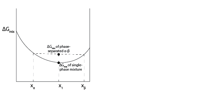
We will define the amount of material in phase \(\beta\) as \(L^\beta\) and the total amount of material in the system as \(F\). We can then write two important tie lines relationships that have graphical interpretations as:

\[\begin{split}\begin{aligned} \frac{L^\beta}{F} &= \frac{x_1 - x_1^\alpha}{x_1^\beta - x_1^\alpha} \\ \Delta G_\textrm{mix} &= \Delta G_\textrm{mix}^\alpha + \frac{\Delta G_\textrm{mix}^\beta - \Delta G_\textrm{mix}^\alpha}{x_1^\beta - x_1^\alpha} \left ( x_1 - x_1^\alpha \right ) \end{aligned}\end{split}\]

The first relationship follows from a mass balance and shows that the amount of material in each phase can be related to the ratio of the line segment from one phase composition to the overall mass fraction normalized by the line segment connecting the two end points; this relationship is called the lever rule and can be applied to any tie line (including tie lines drawn on binary phase diagrams). The second relationship simply expresses the total Gibbs free energy of mixing of a system that separates into two phases as the weighted average of the Gibbs free energy of mixing of each phase (given by the end points of the tie line) and can be interpreted as the equation for the segment of the tie line connecting \(x_\alpha\) and \(x_1\). This relationship thus shows that graphically the intersection of the tie line with the overall mixture composition gives the total Gibbs free energy change of the system if the system were to split into two phases with compositions set by the end points of the tie line.

Using the tie line concept, we can then relate phase compositions to the Gibbs free energy of mixing, building upon concepts in previous lectures.

If we had a phase diagram like that in our figure above, would we expect a single mixed phase or two phases of \(\alpha\) and \(\beta\) to be present at \(x_1\)?

Click for answer

The single, mixed phase (on the curve) has a lower \(\Delta G_{mix}\), so we would see a single, mixed phase.

Let’s consider two other cases:

Case 1:

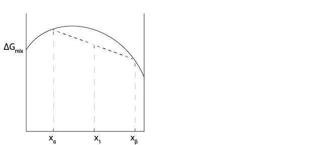
In Case 1, would we expect a single mixed phase or two phases of \(\alpha\) and \(\beta\) to be present at \(x_1\)?

Click for answer

The single, mixed phase (on the curve) has a higher \(\Delta G_{mix}\), so we would see complete phase separation, or demixing. We can infer the amount of each pure system from the tie line.

Case 2: We can now consider the more complicated case where the free energy of mixing has multiple local minima.

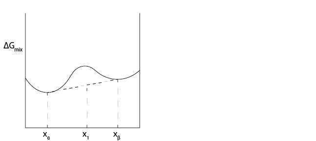
For these plots, there are choices for \(x_{\alpha}\) and \(x_{\beta}\) where any possible tie line will lead to an increase in the free energy, and thus phase separation is not observed. For compositions in between the local minima, we can instead find that tie lines can instead reduce the free energy, implying that phase separation is possible. It can be shown that the tie line that always minimizes the free energy is the

common tangent line

the tie line that is tangent to the free energy curve(s) at two points

The common tangent line concept can also be used when comparing phases on different energy curves – that is, the phases that will be present are those where the slope of the curve(s) are equal. This can be derived by assuming that the conditions of phase equilibrium (i.e. equivalence of chemical potentials or fugacities) are met for the compositions connected by the common tangent line.

Referencing our previous discussion of stability, we can also see that the curvature of the Gibbs free energy of mixing will also have impliciations for mixture stability.

Consider preparing a single-phase mixture with an overall mole fraction that intersects the Gibbs free energy of mixing at a region of the curve that is concave up (\(\left ( \partial ^2\Delta G_\textrm{mix}/\partial x_1^2 \right )_{T,P} > 0\)). Drawing a tie line to any two compositions close to the overall composition - representing small perturbations to the composition of a system that is initially a single phase - will lead to an increase in the free energy, which is unfavorable. Thus, the initially single-phase mixture is stable with respect to small perturbations, or metastable.

Performing the same analysis for a region where the Gibbs free energy is concave down (\(\left ( \partial ^2\Delta G_\textrm{mix}/\partial x_1^2 \right )_{T,P} < 0\)) would show that any perturbation leads to a decrease in the free energy and the overall composition is unstable.

We can therefore define two sets of compositions of interest:

• the compositions connected by a common tangent line that denote the \(\Delta G_{mix}\)-minimizing compositions at equilibrium, and

• the compositions corresponding to inflection points in \(\Delta G_{mix}\) (\(\left ( \partial ^2\Delta G_\textrm{mix}/\partial x_1^2 \right )_{T,P} = 0\)) that denote the transition from metastable to unstable points, or the

limits of stability

inflection points on a \(\Delta G_{mix}\) curve that denote the switch from metastable to unstable mixtures

If we gather up all equilibrium compositions and all limits of stability across a range of temperatures, we yield both the binodal and spinodal curves.

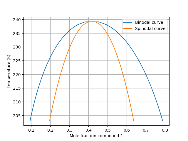Image from COSMO-RS documentation

Some observations:

Unlike VLE, the binodal for LLE does not have to intersect the y-axes as there is typically no liquid-liquid phase transition for most single-component systems

So, what would we see at low pressure / high temperature?

Click for answer

Solid phases.

What would happen if the system is prepared in a single-phase liquid region and then pressurized/cooled to be within the spinodal?

Click for answer

You would rapidly observe segregation of the system into two liquid phases (with compositions defined by the binodal, not the spinodal, since those are the compositions reached at equilibrium) in a process called spinodal decomposition.

What would happen if our conditions were in between the spinodal and binodal lines?

Click for answer

You could observe a metastable single-phase system for a long period of time until eventually phase separation occurs by a process called nucleation and growth, in which a small region of the system spontaneously begins to separate and this regions grows slowly.

Link to Shared Notes