The canonical ensemble

Additional Readings for the Enthusiast

• Chandler [1] Chapter 3.3-3.4

Goals for today’s lecture

• How do we describe systems with fluctuating or non-constant energy?

• How does the breaking the principle of equal a priori change the likelihood of different microstates?

• What is a partition function?

Introduction to the canonical ensemble

In principle, all calculations in statistical mechanics can be performed using the microcanonical ensemble by deriving relationships based on a fixed set of constant energy states. In practice, the microcanonical ensemble is often not convenient because in many cases the energy of the system is not fixed.

For example, most laboratory experiments take place in environments in which the energy of the system is able to exchange with the environment; that is, the walls of the system are diathermal. \(E\) is therefore no longer a fixed quantity and instead varies between each microstate. At equilibrium, however, we know from thermodynamics that the temperature of the system will be equal to the temperature of the environment. It would therefore be ideal to have equations describing systems in which the temperature is fixed in each microstate due to this condition of equilibrium while the energy is allowed to vary.

a repeat definition of the canonical ensemble

The ensemble for which all microstates have a fixed number of particles, volume, and temperature. Also known as the $\(NVT\)$ ensemble.

As we will see, choosing the appropriate ensemble to describe a system of interest is essential in simplifying problem solutions. However, if we allow the energy to vary between each microstate then the probability that a system obtains a given state, \(p_i\), is no longer a constant value - that is, Postulate 2 no longer applies. We thus will derive an expression for the probability of microstate \(i\) in order to calculate ensemble-average quantities for the canonical ensemble.

Let us consider a system of interest that is contact with surroundings that we will refer to as the bath. The bath is significantly larger than the system of interest, so that the energy and number of particles in the bath are also much larger than the energy and number of particles in the system. Thermodynamic parameters associated with the system will be denoted with the subscript \(S\), parameters associated with the bath will be denoted with the subscript \(B\), and parameters associated with the total combination of system and bath will be denoted with the subscript \(T\).

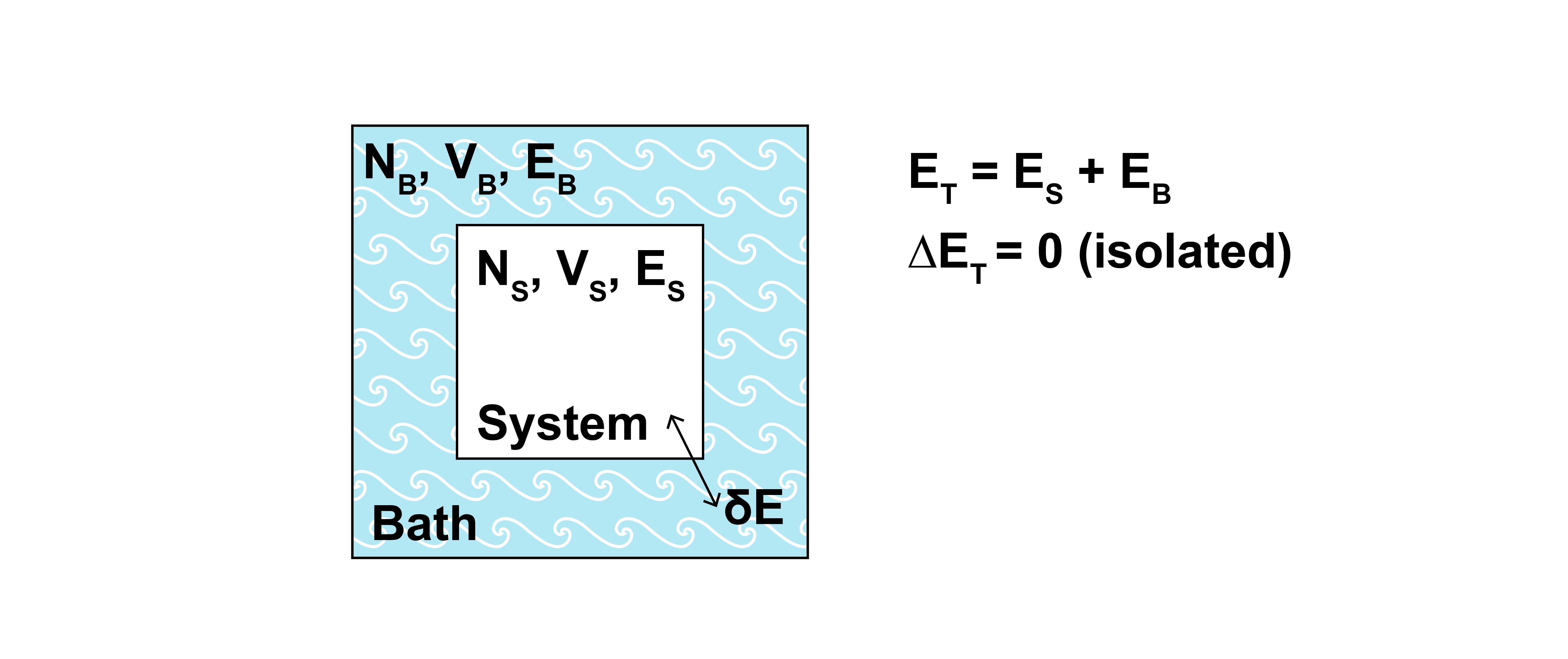
We assume that the walls of the system prevent the exchange of particles and volume so that \(N_S\) and \(V_S\) are fixed; however, the energy, \(E_S\), can exchange with the surrounding bath. At thermal equilibrium, the temperature of the bath and system are equivalent (\(T_S = T_B \equiv T_T\)).

A physical realization of such a system would be a sealed box with conducting walls that allows heat to exchange with the outside environment. Finally, we assume that the total energy, \(E_T\), of the bath plus the system is a constant (i.e., exchanges of energy between the bath and system obey conservation of energy):

\[E_T = E_S + E_B = \text{constant}\]

The total combination of system and bath is isolated.

Does the canonical ensemble refer to the microstates of the system, the bath, or both combined?

[Click for answer]

Microstates of the total isolated system belong to the microcanonical ensemble, but the energy of each of these microstates is partitioned between the system of interest and the bath. The canonical ensemble then refers to the ensemble of microstates describing the system of interest, in which the energy may vary between microstates in the ensemble.

We will now determine the probability \(p_j\) of observing a single microstate of the system, \(j\), which has energy \(E_j\) (noting that there can be many possible microstates with the same energy - in fact, there is a microcanonical ensemble of microstates with the same energy! We use the subscript \(j\) to denote a single specific microstate - that is, a single arrangement of particles with a specific energy \(E_j\) out of the many possible microstates that would have the same energy).

Here, it is useful to frame our experiment in terms of microcanonical ensembles. The set of microstates that correspond to \(E_j\) comprise a microcanonical ensemble (let’s call this Ensemble J), as their energy is equal (as well as \(N\) and \(V\)). The set of microstates for the whole system (bath + system of interest) comprise a microcanonical ensemble, as \(E_T\) is also constant.

So, how many microstates exist within our isolated (total) system that are part of Ensemble J? You could imagine fixing the positions/energies of the \(N_S\) particles into microstate \(j\) and then counting all possible combinations of the positions/energies of the \(N_B\) remaining particles.

This value is equal to the number of microstates of the bath that are possible for the given microstate of the system. Since the energy of the system is fixed and equal to \(E_j\), the energy of the bath is also fixed and equal to \(E_B=E_T-E_j\). Therefore, the bath at energy \(E_B = E_T - E_j\) also constitutes a microcanonical ensemble! Furthermore, our number of states is equal to the degeneracy of a bath microcanonical ensemble with energy \(E_T-E_j\), or \(\Omega(N_B,V_B,E_T-E_j)\).

We could write a similar degeneracy for each possible microstate \(j\) of the system. Since the total isolated system is a microcanonical ensemble in which all microstates are equally probable, the probability of observing a single microstate of the system \(j\) is equal to the number of microstates of the total isolated system in which the system of interest is in microstate \(j\) divided by the total number of microstates of the combined isolated system.

From the logic above, we can write the normalized probability of finding microstate \(j\) of the system in terms of the degeneracy of the bath as:

(16)\[\begin{split}p_j &= \frac{\Omega(N_B, V_B, E_T-E_j)}{\sum_{\textrm{all microstates j}} \Omega(N_B, V_B, E_T-E_j)} \\ &= \frac{\Omega(N_B, V_B, E_T-E_j)}{C_1}\end{split}\]

That is, the probability of finding a particular microstate in the canonical ensemble (of the system) is related to the degeneracy of a bath described by a microcanonical ensemble with energy \(E_T-E_j\). We use the constant \(C_1\) to refer to the normalization factor in the denominator (this quantity will drop out later on in the derivation).

We will proceed from here by relating the degeneracy of the bath microcanonical ensemble to the entropy (following our previous approach) and from there obtaining an expression for \(p_j\) that does not depend on any properties of the bath.

Derivation of canonical partition function

We have just derived the equations for the canonical ensemble, or the ensemble in which every microstate is at the same number of particles, volume, and temperature (\(NVT\)). Unlike the microcanonical ensemble, the energy of each state can vary, and in addition the probability of finding a given state is not necessarily equal. We thus sought to derive the probability of observing a single state in the canonical ensemble, \(p_j\), which has energy \(E_j\).

Why is there not a one-to-one correspondence between energy and microstates in the canonical ensemble?

[Click for answer]

In general, many possible microstates could have the same energy but different microscopic configurations - thus, there is not a one-to-one correspondence between energies and microstates. We will eventually consider the probability of observing one of the many states that have the same energy \(E_\nu\) as opposed to the specific microstate \(j\).

As a reminder, here is our setup:

We now seek to determine \(p_j\). First, we recognize that the total combined system is isolated, so there is a microcanonical ensemble of microstates of the total combined system and the probability of each of these microstates is equal (according to the principle of equal a priori probabilities).

From the logic above, we can write the normalized probability of finding microstate \(j\) of the system in terms of the degeneracy of the bath as (16).

Our goal now is to find an expression for \(p_j\) that does not depend on properties of the bath or total combined system, since in general we only know the properties of the system itself. To begin, we write the logarithm of \(p_j\), recognizing that \(\ln \Omega(N_B, V_B, E_T-E_j)\) is related to the Boltzmann entropy of the bath:

\[\ln p_j = \ln \Omega(N_B, V_B, E_T-E_j) - \ln C_1\]

For these next few lines, I will use the notation \(\Omega_B(E) \equiv \Omega(N_B, V_B, E)\) to simplify the notation.

Show that \(\ln\Omega_B(E_T-E_j) = \ln \Omega_B(E_T) - \frac{E_j}{k_B T_S} + \dots\)

[Show derivation]

By construction, the energy of the bath and the energy of the total combined system is much greater than the energy of the system of interest (\(E_T \gg E_j\)). We can then write a Taylor expansion for \(\ln \Omega(N_B, V_B, E_T-E_j)\) around the point \(E_T-E_j \approx E_T\). Recall that the expression for a Taylor expansion is:

\[\begin{aligned} f(x) &= f(a) + f'(a)(x-a) + \frac{f''(a)}{2!}(x-a)^2 \dots \end{aligned}\]

If I define \(x = E_T-E_j\), \(a = E_T\), and \(x-a = -E_j\), my Taylor expansion for \(\ln \Omega_B(E_T-E_j)\) is

\[\begin{aligned} \ln \Omega_B(E_T-E_j) &\approx \ln \Omega_B(E_T) - E_j \left [\frac{\partial \ln \Omega_B(E_T-E_j)}{\partial (E_T-E_j)} \right ]_{N_B, V_B} + \dots \end{aligned}\]

To simplify this equation, we substitute in the expression for the Boltzmann entropy of the bath microcanonical ensemble, \(S_B(E_T - E_j) = k_B \ln \Omega_B(E_T - E_j)\):

\[\begin{aligned} \ln \Omega_B(E_T-E_j) &\approx \ln \Omega_B(E_T) - \frac{E_j}{k_B} \left [ \frac{\partial S_B(E_T-E_j)}{\partial (E_T-E_j)} \right ]_{N_B, V_B} + \dots \end{aligned}\]

Next, we recognize that \(\left ( \frac{\partial S_B(E_T-E_j)}{\partial (E_T-E_j)}\right )_{N_B, V_B} = \frac{1}{T_B}\) using the same thermodynamic relation from last lecture, and moreover \(1/T_B = 1/T_S\) due to the equilibrium between the system and bath:

\[\begin{split}\begin{aligned} \ln \Omega_B(E_T-E_j) &\approx \ln \Omega_B(E_T) - \frac{E_j}{k_B T_B} + \dots \\ &= \ln \Omega_B(E_T) - \frac{E_j}{k_B T_S} + \dots \end{aligned}\end{split}\]

What happens to the higher-order terms?

[Click for answer]

The next highest order term would be of the form:

\[\begin{aligned} \left ( \frac{\partial^2 S_B}{\partial E_B^2} \right ) &= \left ( \frac{\partial (1/T_B)}{\partial E_B} \right ) \propto \frac{1}{C_V} \end{aligned}\]

Thus, the second order term is related to the inverse of the heat capacity of the bath; we can assume that this value is negligible if the bath is large (i.e., the temperature of the bath is a constant). This is an assumption about the bath/combined system only, and thus is not violated even if our system of interest is small!

We can now use this Taylor expansion, truncated at first order, to write a new expression for the probability of obtaining a system in microstate \(j\):

\[\begin{split}\begin{aligned} \ln p_j &= \ln \Omega_B(E_T) - \frac{E_j}{k_B T_S} - \ln C_1 \\ p_j &= \frac{\Omega_B(E_T)}{C_1} e^{-E_j/k_BT_S} \\ \therefore p_j &= C_2 e^{-E_j/k_BT_S} \end{aligned}\end{split}\]

Here, \(C_2\) is a constant the combines the degeneracy of the bath for some given energy, \(\Omega_B(E_T)\), with the normalization constant \(C_1\). The value \(C_2\) is equivalent for all microstates because it is a property of our combined system, including the fictitious bath.

We can now identify an expression for \(C_2\) by requiring that \(\sum_j p_j = 1\) to normalize the probability distribution:

\[\begin{split}\begin{aligned} \sum_j^{\textrm{microstates}} p_j &= \sum_j^{\textrm{microstates}} C_2 e^{-E_j/k_BT_S} = C_2 \sum_j^{\textrm{microstates}} e^{-E_j/k_BT_S} = 1 \\ C_2 &= \frac{1}{\sum_j e^{-E_j/k_BT_S}}\\ \therefore & p_j = \frac{e^{-E_j/k_BT_S}}{\sum_j e^{-E_j/k_BT_S}} \end{aligned}\end{split}\]

canonical partition function

A term, here \(Z \equiv \sum_j e^{-E_j/k_BT}\), that normalizes the probability of finding state \(j\) in the canonical ensemble.

Boltzmann factor / Boltzmann weight

The weighting term for each state, \(e^{-E_j/k_BT}\) that communicates the energetic favorability of that state.

At this point no parameters related to the bath or total combined system remain in the expression for \(p_j\) - the probability of identifying a microstate in the canonical ensemble is related entirely to the system properties without any contribution from the bath as desired. We will henceforth drop all \(S\) and \(B\) subscripts from system properties since \(N\), \(V\), and \(T\) are no longer ambiguous. The partition function is then:

\[\begin{split}\begin{aligned} Z &= \sum_j^{\textrm{all states}} e^{-E_j /k_B T} \\ p_j &= \frac{e^{-E_j/k_BT}}{Z} \end{aligned}\end{split}\]

The factor \(k_B T\) is essentially a scaling factor and is the amount of thermal energy accessible to the system. This expression shows that the probability that a system samples a particular microstate is related to the relative values of \(E_j\) and \(k_B T\). Often, we will also define \(\beta \equiv 1/k_B T\) to simplify notation.

Conceptually, why does it make sense that the probabilities are exponentially weighted?

[Click for answer]

States with low (negative) energies are exponentially more probable than high energy states. If the energy of a state is much larger than \(k_B T\), the probability of observing that state is very low. Conversely, if the temperature of a system is very high, the probability of any given state becomes approximately equal since variations in \(E_j\) between states will be negligible relative to the value of \(k_BT\).

So far, we have focused on the energy of a particular microstate, referring to a particular set of particle configurations and energies. We can also write the probability \(p_\nu\) of obtaining any microstate of the system of interest that has an energy \(E_\nu\). In general, there are many possible microstates that have the same energy, but have different particle configurations. The number of such states is given by the microcanonical degeneracy \(\Omega(N_S, V_S, E_\nu)\), so \(p_\nu \gg p_j\). \(p_\nu\) is equal to the probability that the system of interest is in a particular microstate with energy \(E_j\) (where the value of \(E_j = E_\nu\)) multiplied by the number of possible microstates of the system for which \(E_j = E_\nu\). This gives (again, dropping all subscripts now):

\[\begin{split}\begin{aligned} p_\nu &= \Omega(N,V, E_\nu) p_j \\ &= \frac{\Omega(N, V, E_\nu) e^{-\beta E_\nu}}{\sum_\nu^\textrm{energies} \Omega(N, V, E_\nu) e^{-\beta E_\nu}} \label{canonical_probability} \end{aligned}\end{split}\]

Here, the denominator is again obtained by normalizing the expression in the numerator. Since the sums in the denominators of the expressions for both \(p_j\) and \(p_\nu\) run over all possible states, both are equivalent. Thus, we can write the partition function of the system as:

\[Z = \sum_j^{\text{microstates}} e^{-\beta E_j} = \sum_\nu^{\text{energies}} \Omega(N, V, E_\nu) e^{-\beta E_\nu} \label{canonical_probability2}\]

where again the first form has a sum that runs over all individual microstates (indicated by the subscript \(j\)) while the second form has a sum that runs over all possible energy levels (indicated by the subscript \(\nu\)) and includes the degeneracy associated with each energy level. The partition function is a constant which normalizes the probabilities, and since it enumerates all possible microstates of the system (each weighted by a corresponding Boltzmann factor), the value of the partition function is the same regardless of whether we sum over microstates or over energy levels. We will next connect the partition function to macroscopic thermodynamic parameters.

Connecting the canonical ensemble to thermodynamics

Just as we can use the relation \(S = k_B \ln \Omega(N, V, E)\) to derive relationships between the degeneracy in the microcanonical ensemble and various thermodynamic variables through the entropy, we can relate the canonical partition function to the Helmholtz free energy using the relation:

\[\begin{aligned} F &= -k_B T \ln Z (N, V, T) \end{aligned}\]

We will show this by first deriving an expression for the ensemble-average energy of the canonical ensemble using the expression for the partition function. We will then show that invoking the relation \(F=-k_BT \ln Z\) allows us to equate the ensemble-average energy to the thermodynamic relationship between the internal energy and the Helmholtz free energy. First, we can write an expression for the ensemble-average energy of the canonical ensemble:

\[\begin{split}\begin{aligned} \langle E \rangle &= \sum_j^\text{states} p_j E_j \\ &= \sum \left ( \frac{e^{-\beta E_j}}{Z} \right ) E_j \\ &= \frac{1}{Z} \sum_j E_j e^{-\beta E_j} \end{aligned}\end{split}\]

Here, we have used the expression for the probability of finding a particular microstate in the canonical ensemble, \(p_j \equiv e^{-\beta E_j}/Z\). We proceed by recognizing that the \(E_je^{-\beta E_j} = -\frac{\partial}{\partial\beta}e^{-\beta E_j}\), allowing us to write:

\[\begin{split}\begin{aligned} \langle E \rangle &= \frac{1}{Z} \sum_j - \frac{\partial}{\partial \beta} \left (e^{-\beta E_j} \right)_{N,V} \\ &= -\frac{1}{Z} \frac{\partial}{\partial \beta} \left (\sum_j e^{-\beta E_j}\right )_{N,V} \label{distributive_de} \\ &= - \frac{1}{Z} \left ( \frac{\partial Z}{\partial \beta}\right )_{N,V} \\ &= - \left(\frac{\partial \ln Z}{\partial \beta} \right )_{N,V} \end{aligned}\end{split}\]

Note that we have used a few tricks to get this last result - specifically, we note that a sum of derivatives is equivalent to the derivative of a sum (\(\sum \frac{\partial X_j}{\partial Y} = \frac{\partial}{\partial Y}\sum X_j\)) and this sum is equivalent to the partition function, then we use the chain rule to arrive at the final result, which expresses the ensemble-average energy in terms of a temperature deriative of the partition function (since \(\beta = 1/k_B T\), a derivative with respect to \(\beta\) is equivalent to a derivative with respect to inverse temperature).

So far we have assumed no connection to thermodynamics at all. We now show that deriving an equivalent expression for the internal energy in terms of a temperature derivative of the Helmholtz free energy allows us to relate the Helmholtz free energy to the partition function. Let us now consider the thermodynamic relationship between the Helmholtz free energy and internal energy from a few lectures ago:

\[\begin{aligned} F = E -TS \end{aligned}\]

We can also write the total derivative of the Helmholtz free energy (and substitute in the fundamental relation for \(dE\)) to obtain a relationship for the entropy to eliminate it from the expression above:

\[\begin{split}\begin{aligned} dF &= dE - TdS - SdT \\ dE &= TdS - PdV + \mu dN \\ dF &= -S dT - PdV + \mu dN \\\label{dF} &= \left ( \frac{\partial F}{\partial T} \right )_{N,V} dT + \left ( \frac{\partial F}{\partial V} \right )_{N, T} dV + \left ( \frac{\partial F}{\partial N} \right )_{V, T} dN \end{aligned}\end{split}\]

This expression then yields:

\[\begin{split}\begin{aligned} S &= -\left ( \frac{\partial F}{\partial T}\right )_{N,V} \\ \therefore E &= F - T \left ( \frac{\partial F}{\partial T}\right )_{N,V} \end{aligned}\end{split}\]

Letting \(T = k_B/\beta\) we can write:

\[\begin{split}\begin{aligned} E &= F - \frac{k_B}{\beta} \left ( \frac{\partial F}{\partial (k_B/\beta)}\right )_{N,V} \\ %&= F - \frac{1}{\beta} \left ( \frac{\partial F}{\partial \beta}\right )_{N,V} \left ( \frac{\partial %\beta}{\partial \beta^{-1}}\right )_{N,V} \\ &= F + \beta \left ( \frac{\partial F}{\partial \beta}\right )_{N,V} \end{aligned}\end{split}\]

We now have the two following expressions, one derived from the canonical ensemble and one from thermodynamics:

\[\begin{split}\begin{aligned} \langle E \rangle &= - \left(\frac{\partial \ln Z}{\partial \beta} \right )_{N,V} \quad \text{stat. mech} \\ E &= F + \beta \left ( \frac{\partial F}{\partial \beta}\right )_{N,V} \quad \text{thermo} \end{aligned}\end{split}\]

From ergodicity, we also know that \(\langle E \rangle = E\), meaning that the ensemble-average value of \(E\) calculated from statistical mechanics is equivalent to the thermodynamic definition. We could equate these expressions to find an expression for \(F\), noting the visual similarity of our thermodynamic definition to the product rule. Doing so would lead to:

\[\begin{aligned} F &= -k_B T \ln Z = -(1/\beta) \ln Z \end{aligned}\]

We can confirm this relationship by substituting it into the first expression to check for consistency:

\[\begin{split}\begin{aligned} \langle E \rangle &= \left(\frac{\partial (\beta F)}{\partial \beta} \right )_{N,V} \\ &= F + \beta \left ( \frac{\partial F}{\partial \beta}\right )_{N,V} \\ &= E \quad \text{ from thermo} \end{aligned}\end{split}\]

Therefore, substituting in our putative link between the partition function and the Helmholtz free energy correctly derives the same expression obtained from thermodynamics alone (given the equivalence between ensemble-average energy and macroscopic energy according to Postulate 1). This confirms the relationship between the Helmholtz free energy and the canonical partition function. To summarize, our three critical relationships for the canonical ensemble are then:

\[\begin{split}\begin{aligned} Z &= \sum_j^{\text{microstates}} e^{-\beta E_j} = \sum_\nu^{\text{energies}} \Omega(N,V,E_\nu) e^{-\beta E_\nu}\\ p_j &= \frac{e^{-\beta E_j}}{Z} \\ F &= -k_B T \ln Z(N,V,T) \end{aligned}\end{split}\]

Revisiting the two-state system

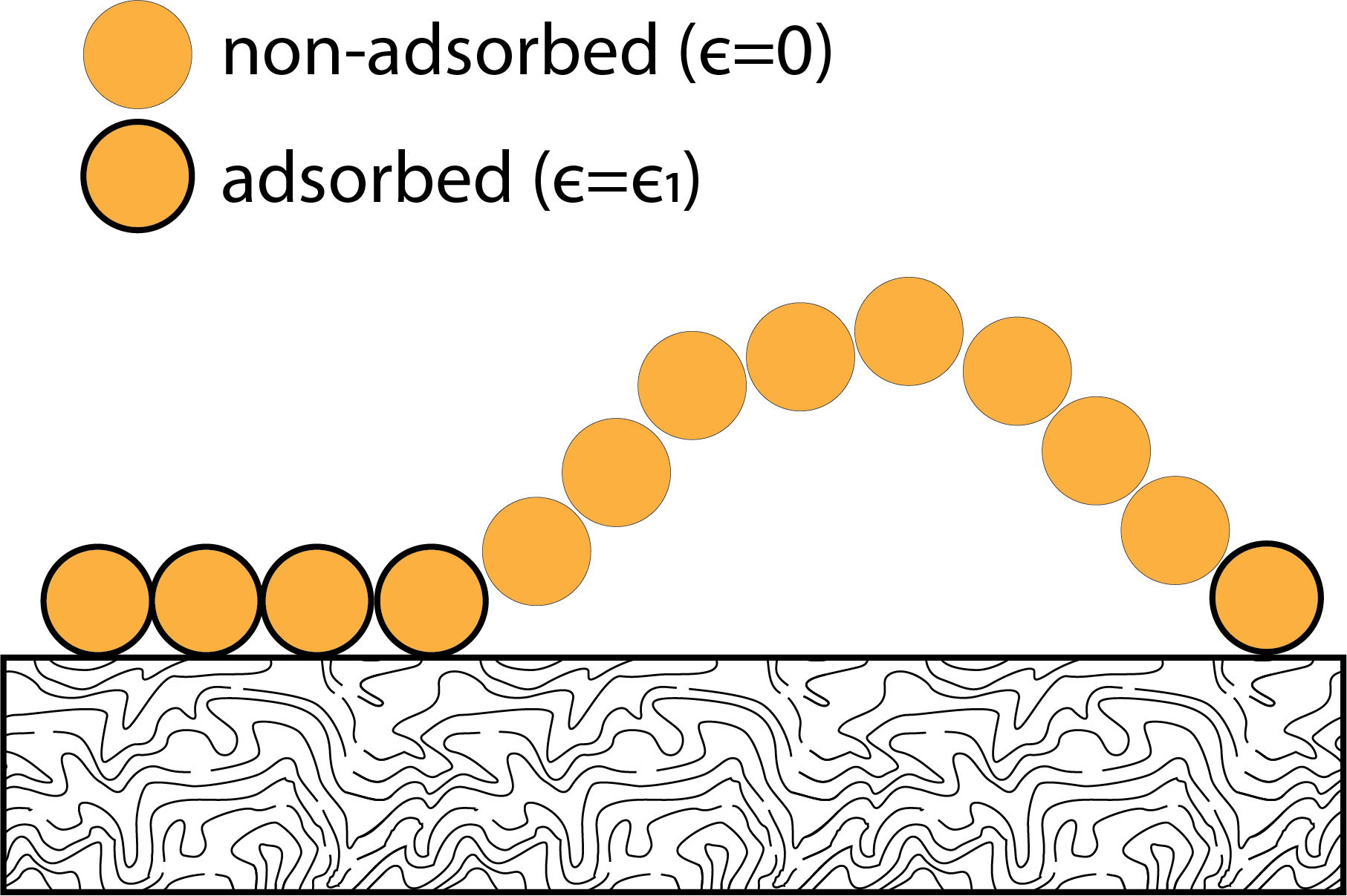
To illustrate how a judicious choice of statistical ensemble can simplify the analysis of systems, we will repeat the example from our previous lecture using the canonical ensemble, instead of the microcanonical ensemble. Recall that the system under consideration is a polymer adsorbed to a surface with \(N\) total monomers in the chain, of which \(n\) are adsorbed to the surface with an energy \(-\epsilon\). The total energy of the system is then \(E = -n \epsilon\) and we seek to relate the number of adsorbed monomers to the temperature.

Previously, we solved this problem using the microcanonical ensemble by first solving for the relationship between the entropy, \(S\), and the number of adsorbed monomers, then identifying a temperature dependence via derivative of the entropy. If we instead treat the system using the canonical ensemble by assuming that the energy of the system is allowed to vary (i.e., the number of adsorbed monomers varies) and only the temperature is held fixed, we can directly relate temperature to energy. We will solve this problem in two ways.

In our first approach, we recognize that all monomers adsorb independently of each other. Since the monomers are independent, the probability that one monomer adsorbs does not affect the probability that another monomer adsorbs. Therefore, we can instead consider a single monomer as a system, in which case the canonical ensemble for a single monomer has only two microstates: either adsorbed or not adsorbed. For a single monomer we can write that the probability \(\rho\) of adsorbing in the canonical ensemble is:

\[\begin{split}\begin{aligned} \rho &= \frac{e^{-\beta E_\textrm{adsorb}}}{\sum_j^\text{microstates} e^{-\beta E_j}} \\ &= \frac{e^{\beta \epsilon}}{e^{-\beta(0)} + e^{\beta(\epsilon)} } \\ &= \frac{e^{\beta \epsilon}}{1 + e^{\beta\epsilon}} \end{aligned}\end{split}\]

Here, we have explicitly enumerated both states in the partition function. The ensemble-average number of adsorbed monomers is then:

\[\begin{split}\begin{aligned} \langle n \rangle &= \sum_{states} \rho = N \rho \\ &= \frac{ N e^{\beta \epsilon}}{1 + e^{\beta\epsilon}} \\ &= \frac{N}{1 + e^{-\beta\epsilon}} \end{aligned}\end{split}\]

This result is the same expression that was derived using the microcanonical ensemble and is obtained much more easily.

Note the key steps: we assume that the monomers are independent, we calculate the probability of adsorbing for each monomer, then multiply this probability by the number of monomers. This assumption of independent treatment of a set of identical systems will be discussed further in future lectures.

We can also obtain this result directly from the canonical partition function. Here we will use \(z\) to represent the partition function for adsorbing a single monomer (with two terms as above) and let \(\langle \epsilon \rangle\) be the ensemble-average energy per monomer. The ensemble-average number of adsorbed monomers is then \(\langle n \rangle = -N \langle \epsilon \rangle / \epsilon\). Using a relation from above we can then write:

\[\begin{split}\begin{aligned} \langle \epsilon \rangle &= -\left(\frac{\partial \ln z}{\partial \beta} \right )_{N,V} \\ &= -\left ( \frac{\partial \ln (1 + e^{\beta\epsilon})}{\partial \beta} \right )_{N, V} \\ &= -\frac{\epsilon e^{\beta \epsilon}}{1+e^{\beta \epsilon}} \\ \langle n \rangle &= -N \langle \epsilon \rangle / \epsilon \\ &= \frac{N }{1 + e^{-\beta \epsilon}} \label{eq:3.37} \end{aligned}\end{split}\]

This approach again returns the same result.

Link to Shared Notes