Nuances of stochastic sampling in statistical ensembles

Additional Readings for the Enthusiast

• Frenkel and Smit [2], Ch. 3

Goals for Today’s Lecture

• Understand the need for non-random sampling in statistical ensemble

• Describe Markov chains, importance sampling, detailed balance

• Derive the acceptance criteria for the Metropolis-Hasting algorithm

Importance sampling

One major hitch up to this point has been our probability distribution – in the area example, we directly sampled this by selecting points at random. In our determinate equations, we had it predetermined.

To evaluate ensemble averages from the canonical ensemble, we can choose our probability density, \(p(x)\), to maximize the likelihood of sampling configurations that contribute meaningfully to the calculation of the ensemble average. This is the essence of

importance sampling

sampling from a distribution of states in order to maximize the information gained from each observation

First, let’s recall that the probability of finding the system in a given microstate of the canonical ensemble, \(p(\textbf{r}^N)_{NVT}\), is related to the Boltzmann factor for that state normalized by the partition function. We can then write:

\[\begin{split}\begin{aligned} p(\textbf{r}^N)_{NVT} &= \frac{\exp \left [-\beta E(\mathbf{r}^N)\right ]}{Z} \\ \langle Y \rangle_{NVT} &= \int d \mathbf{r}^N p(\textbf{r}^N)_{NVT} Y(\mathbf{r}^N) \end{aligned}\end{split}\]

The ensemble average then has the same form as \(F = \int_a^b f(x) dx\) if we let \(f(x) = p(\mathbf{r}^N)_{NVT} Y(\mathbf{r}^N)\). Following the reasoning above, we can then approximate \(\langle Y \rangle_{NVT}\) by:

\[\begin{aligned} \langle Y \rangle_{NVT} = \left \langle \frac{ p(\mathbf{r}^N)_{NVT} Y(\mathbf{r}^N) }{p(\mathbf{r}^N)} \right \rangle_{\textrm{trials}} \end{aligned}\]

From this expression, we see that if we select trials according to the probability distribution \(p(\mathbf{r}^N) = p(\mathbf{r}^N)_{NVT}\), then we get:

\[\langle Y \rangle_{NVT} = \langle Y \rangle_{\textrm{trials}} \label{ensemble_average_mc}\]

Thus, we choose configurations in our ensemble according to the canonical ensemble probability distribution, in which case the ensemble-average value of \(Y\) can be estimated by sampling configurations according to their Boltzmann weight. Finally, we note that we just need to know the probability of sampling a configuration - we do not necessarily need an expression for the partition function itself.

Our problem then boils down to: how do we select states according to the correct probability distribution without knowing the value of the partition function?

Markov chains

To do so, we will generate a

Markov chain of states

a sequence of states that is determined one step at a time based upon the probability moving from one state to another

A Markov chain satisfies the following two conditions:

• Each state generated belongs to a finite set of possible outcomes called the state space. The statistical mechanical analogue to this statement is to say that each microstate generated belongs to a finite ensemble. We can denote each possible state by \(\mathbf{r}_1^N, \mathbf{r}_2^N, \mathbf{r}_3^N, \dots\) for the enormous set of possible microstates within the canonical ensemble that we are sampling. For the canonical ensemble, this state space is equal to \(V^N\), the accessible phase space.

• The probability of sampling state \(i+1\) in the sequence of states sampled depends only on state \(i\), and not on previous states in the chain.

Since the likelihood of sampling a new state is only related to what current state we are in, we can define a transition probability, \(\Pi(m\rightarrow n)\), which defines the likelihood of transitioning from state \(m\) to state \(n\). We can then imagine an algorithm in which we start in some state \(m\) then transition to a new state \(n\) with a probability given by \(\Pi(m\rightarrow n)\) and repeat this for a large number of trials.

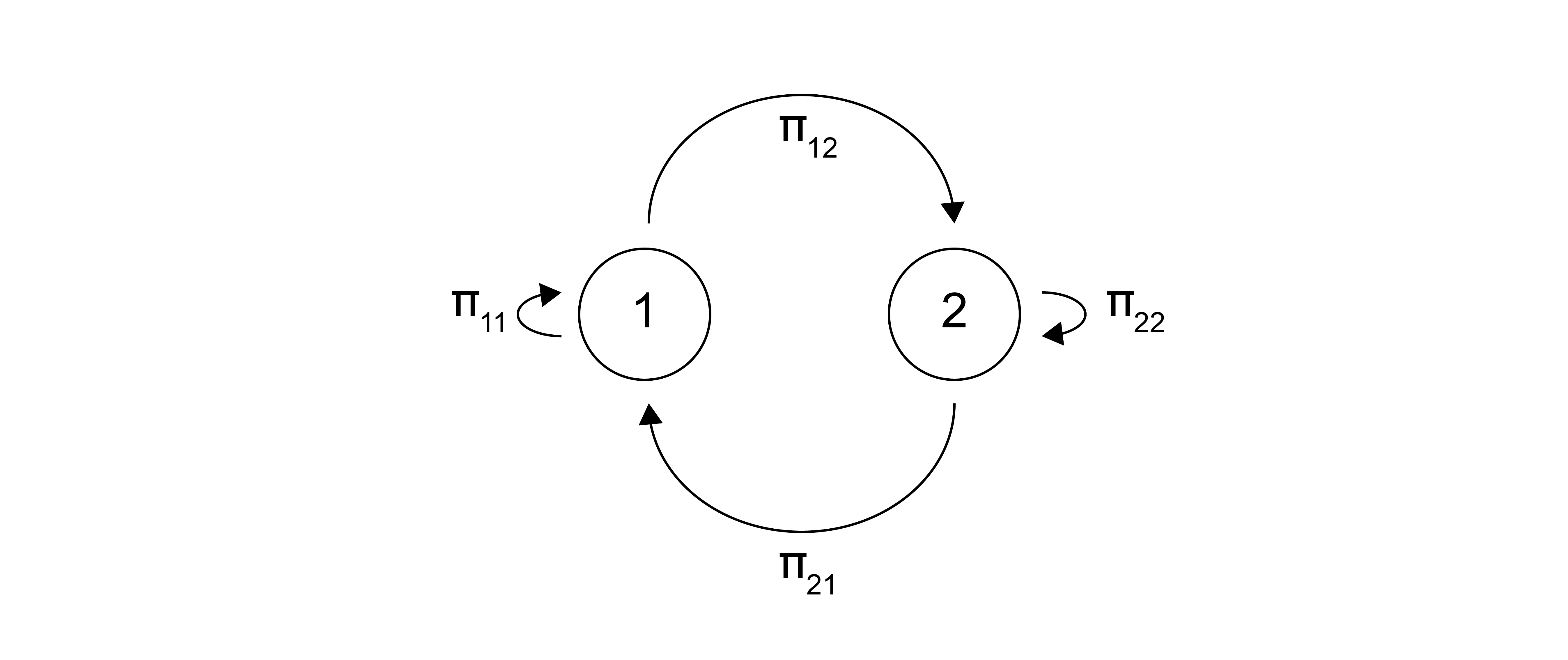
If we do this an infinite number of times, then the state \(m\) will appear with an overall probability given by \(p(m)\), where \(p(m)\) is the limiting probability distribution that does not depend on any of the other states (unlike the transition probability). When sampling from the canonical ensemble, then, we want \(p(m)\) to equal \(p(\mathbf{r}_m^N)_{NVT}\) - that is, the likelihood of sampling state \(m\) if we take enough states from our Markov chain is equal to the probability of sampling that state according to the canonical ensemble distribution function. Thus, we need to find an expression for the transition probability, \(\Pi\), that yields this correct limiting distribution.

Detailed balance

At equilibrium, the probability of finding the system in a configuration \(\mathbf{r}_m^N\) must be stationary, meaning that the probability distribution of the canonical ensemble is invariant with time (this is a consequence of ergodicity) and is equal to the limiting distribution of our Markov chain. If we think about a Markov chain as a very large sequence of states, then for the probability of a particular state to be stationary, the number of transitions into that state must be the same as the number of transitions out of it.

Think of this like a mass balance in transport - the flux into a particular state is equal to the flux out of it, otherwise we would “accumulate” probability for that state. Therefore, it must be the case that in any given Markov chain the number of trials that generate new states from a particular state must be equal to the total number of trials from all other states that generate the original configuration.

If we write the probability of transitioning from some configuration \(\mathbf{r}_m^N\) to \(\mathbf{r}_n^N\) as \(\Pi(\mathbf{r}_m^N \rightarrow \mathbf{r}_n^N)\) and the probability of being in state \(\mathbf{r}_m^N\) as \(p(\mathbf{r}_m^N)\), then we can fulfill the condition that \(p(\mathbf{r}_m^N)\) is stationary by imposing the condition of

detailed balance

\[p(\mathbf{r}_m^N) \Pi(\mathbf{r}_m^N \rightarrow \mathbf{r}_n^N) = p(\mathbf{r}_n^N) \Pi(\mathbf{r}_n^N \rightarrow \mathbf{r}_m^N)\]

We can rearrange this expression to write:

\[\frac{p(\mathbf{r}_m^N)}{p(\mathbf{r}_n^N)} = \frac{ \Pi(\mathbf{r}_n^N \rightarrow \mathbf{r}_m^N)}{\Pi(\mathbf{r}_m^N \rightarrow \mathbf{r}_n^N)}\]

Writing detailed balance in this form more clearly shows the consequence of this definition - if the probability of state \(m\), \(p(\mathbf{r}_m^N)\), is 10 times larger than the probability of state \(n\), then this expression says that there will be 10 times more transitions from state \(n\) to \(m\) than transitions from \(m\) to \(n\), agreeing with expectations. Enforcing this condition for all possible pairs of states guarantees that the number of transitions into and out of each state is equal if an infinite number of transitions are attempted (detailed balance is actually an overly stringent criterion - we could achieve the same properties while enforcing a less stringent relationship between transition probabilities, but that is outside the scope of this class).

If a system obeys detailed balance, then the Markov chain must reach a stationary probability distribution which is necessarily true for any equilibrium system.

The Metropolis-Hastings algorithm

Having defined the principle of detailed balance, we can now apply this to a particular Markov chain that samples states within the canonical ensemble by following the

Metropolis-Hastings algorithm

Also known as the “Metropolis algorithm”. An algorithm that samples states using acceptance criteria based upon transition probabilities.

The key aspect of the Metropolis algorithm is to further divide the transition probability, \(\Pi(\mathbf{r}_m^N \rightarrow \mathbf{r}_n^N)\), into two terms - the probability of generating a new trial state, \(g(\mathbf{r}_m^N \rightarrow \mathbf{r}_n^N)\), and the probability of accepting the new trial state, \(\alpha (\mathbf{r}_m^N \rightarrow \mathbf{r}_n^N)\):

\[\Pi(\mathbf{r}_m^N \rightarrow \mathbf{r}_n^N) = g(\mathbf{r}_m^N \rightarrow \mathbf{r}_n^N) \alpha(\mathbf{r}_m^N \rightarrow \mathbf{r}_n^N)\]

Show that, in the canonical ensemble, \(\frac{\alpha(\mathbf{r}_m^N \rightarrow \mathbf{r}_n^N)}{\alpha(\mathbf{r}_n^N \rightarrow \mathbf{r}_m^N)} = \exp \left \{ -\beta \left [ E(\mathbf{r}_n^N) - E(\mathbf{r}_m^N) \right ] \right \}\).

Show derivation

Given the preceding definition, the equation for detailed balance can then be rewritten as:

\[\begin{aligned} \frac{g(\mathbf{r}_m^N \rightarrow \mathbf{r}_n^N) \alpha(\mathbf{r}_m^N \rightarrow \mathbf{r}_n^N)}{g(\mathbf{r}_n^N \rightarrow \mathbf{r}_m^N) \alpha(\mathbf{r}_n^N \rightarrow \mathbf{r}_m^N )} &= \frac{p(\mathbf{r}_n^N)}{p(\mathbf{r}_m^N)} \end{aligned}\]

Now, we can connect this expression explicitly to the canonical ensemble. In the canonical ensemble, the probability of finding a particular state \(m\) is related to that state’s Boltzmann weight, so we can write:

\[p(\mathbf{r}_m^N)_{NVT} = \frac{\exp \left [ -\beta E(\mathbf{r}_m^N) \right ]}{Z}\]

Next, we assume that the probability \(g\) for generating trial moves is symmetric, and then write that \(g(\mathbf{r}_m^N \rightarrow \mathbf{r}_n^N) = g(\mathbf{r}_n^N \rightarrow \mathbf{r}_m^N)\). We can assume this because in general we can arbitrarily choose a function for \(g\) as long as the detailed balance condition is satisfied. Combining these expressions, we then write:

\[\begin{split}\begin{aligned} \frac{g(\mathbf{r}_m^N \rightarrow \mathbf{r}_n^N) \alpha(\mathbf{r}_m^N \rightarrow \mathbf{r}_n^N)}{g(\mathbf{r}_n^N \rightarrow \mathbf{r}_m^N) \alpha(\mathbf{r}_n^N \rightarrow \mathbf{r}_m^N )} &= \frac{p(\mathbf{r}_n^N)_{NVT}}{p(\mathbf{r}_m^N)_{NVT}} \\ \frac{\alpha(\mathbf{r}_m^N \rightarrow \mathbf{r}_n^N)}{\alpha(\mathbf{r}_n^N \rightarrow \mathbf{r}_m^N)} &= \exp \left \{ -\beta \left [ E(\mathbf{r}_n^N) - E(\mathbf{r}_m^N) \right ] \right \} \end{aligned}\end{split}\]

This equation stipulates the conditions on the acceptance condition, \(\alpha(\mathbf{r}_m^N \rightarrow \mathbf{r}_n^N)\), that leads to correct Boltzmann-weighted sampling of configurations in the canonical ensemble. Importantly, the partition function drops out of this expression, resolving the issue of being unable to calculate the partition function explicitly. In principle, several choices of the acceptance condition could fulfill the conditions imposed detailed balance; the choice used in the original derivation of the Metropolis algorithm is:

(23)\[\alpha(\mathbf{r}_m^N \rightarrow \mathbf{r}_n^N) = \text{min} \left ( 1, \exp \left \{ -\beta \left [ E(\mathbf{r}_n^N) - E(\mathbf{r}_m^N) \right ] \right \} \right )\]

which fulfills our earlier condition.. This is apparent if we consider the case where \(p(\mathbf{r}_n^N) < p(\mathbf{r}_m^N)\), then:

• \(E(\mathbf{r}_n^N) - E(\mathbf{r}_m^N) > 0\)

• \(\exp \left \{ -\beta \left [ E(\mathbf{r}_n^N) - E(\mathbf{r}_m^N) \right ] \right \} < 1\)

• \(\alpha(\mathbf{r}_m^N \rightarrow \mathbf{r}_n^N) = \exp \left \{ -\beta \left [ E(\mathbf{r}_n^N) - E(\mathbf{r}_m^N) \right ] \right \}\)

• \(\alpha(\mathbf{r}_n^N \rightarrow \mathbf{r}_m^N) = 1\)

If the proposed state has a lower energy than our current one, what is the probability we will accept the transition move?

Click for answer

The probability is 1. All transitions in which the system energy is lowered are automatically accepted.

It is possible for the system to stay in the same state; that is:

\[\Pi(\mathbf{r}_m \rightarrow \mathbf{r}_m) = 1 - \sum_{n\ne m} \Pi(\mathbf{r}_m \rightarrow \mathbf{r}_n)\]

Any given Markov chain generated using the Metropolis Monte Carlo algorithm can thus have many consecutive identical states, particularly if the system reaches a local energy minimum.

Based on this derivation, the Metropolis Monte Carlo algorithm for correctly sampling states from the canonical ensemble consists of the following steps (given in Problem Set 2):

1. Assume the system is in a configuration, \(\mathbf{r}_m^N\), which is state \(i\) in a Markov chain.

2. Generate a trial configuration \(\mathbf{r}_n^N\) according to the probability \(g(\mathbf{r}_m^N \rightarrow \mathbf{r}^N_n)\). There can be many possible ways of generating trial configurations (or many “moves”), as noted below.

3. Calculate the energy difference between the new and old configurations and calculate the probability of transitioning to the new state, \(\alpha(\mathbf{r}_m^N \rightarrow \mathbf{r}_n^N)\) according to Eq. (23).

4. Generate a uniform random number in the range [0, 1]. If the random number is less than the transition probability, then state \(i +1\) in the Markov chain has the new configuration \(\mathbf{r}_n^N\) and the system configuration is updated; that is, the new trial move is accepted. If the random number is greater than the transition probability, then state \(i+1\) in the Markov chain has the old configuration (\(\mathbf{r}_m^N\)), the system configuration remain the same, and the move is rejected. This step is the stochastic implementation of Eq.(23).

5. Repeat steps 2-4 until a sufficient number of states in the Markov chain are generated.

6. Approximate the ensemble-average value of some observable \(Y(\mathbf{r}^N)\) by averaging over all states in the Markov chain. Note that many states will be repeated, and we include consecutive identical states (which appear when moves are rejected). Averaging over all states in the Markov chain then calculates \(\langle Y(\mathbf{r}^N)\rangle_{NVT}\).

Metropolis Monte Carlo has several advantages. First, the acceptance ratio only relies on the energies of the two states, and as a result the rule for generating trials moves with a probability given by \(g\) can be arbitrary and does not have to be physically meaningful. For example, typical trial moves in a system consisting of a series of liquid-like particles could be the slight displacement of a single particle, the rotation of an entire molecule, the displacement of several particles simultaneously, or non-physical moves such as “hopping” a particle from one side of the system to the other.

This feature also means that many-body potentials can be easily used to calculate system energies, which is more difficult to do in molecular dynamics simulations that require pair potentials. In addition, because all configurations are sampled according to their equilibrium probability distributions, averaging observables over simulation configurations generates ensemble averages. The downside, however, is that the algorithm is only useful for calculating equilibrium thermodynamic properties and not observing system kinetics.

Some care has to be taken in computing ensemble-average quantities. One choice that can affect values is the starting configuration. If an initial configuration is generated that is a high energy (and thus unlikely) state, then it may contribute to a large degree to a resulting ensemble average even if its actual Boltzmann weight is low. In other words, imagine a chain with only 10 states; the initial state will contribute to 1/10 of the ensemble-average even if it should actually contribute to a much smaller degree. As a result, it is typical to run a MC algorithm for an initial period of steps that are treated as an “equilibration” period so that any unphysical, high energy starting configuration relaxes to a set of low-energy configurations. Inspection of the MC equations indeed shows that there should generally be a decrease in the system energy until a set of configurations with similar low-energy values are obtained.

Link to Shared Notes