Conditions of equilibrium

Additional Readings for the Enthusiast

Tester and Modell [4], Ch. 5.3, 5.5, 6.2-6.4, Appendix A, Appendix C

Goals for Today’s Lecture

• Understand the behavior of arbitrary thermodynamic potentials at equilibrium

• Define the path of a state variable between two states given an arbitrary set of variables

• Relate derivatives of thermodynamic potentials using Maxwell relations

• Apply the Euler theorem to obtain the Gibbs-Duhem equation

Behavior of new thermodynamic potentials at equilibrium

In the last lecture, we introduced the Legendre transform which expresses a function in terms of its tangent lines and their intercepts. The Legendre transform of a function in which \(k\) variables are transformed is given by (31):

\[y^{(k)} = y^{(0)} - \sum_i^k q_i x_i\]

Here, \(q_i\) is a first-order partial derivative of \(y^{(0)}\) and \(x_i\) is its conjugate independent variable. We used Legendre transforms of the fundamental relation to derive expressions for new thermodynamic potentials (free energies) that are a function of experimentally accessible independent variables. For example, the Gibbs free energy is the second Legendre transform of the fundamental relation in the energy representation for which the independent variables \(\underline{S}\) and \(\underline{V}\) are replaced by the conjugate variables \(T\) and \(-P\), which are the slopes of tangent lines to the surface specified by the fundamental relation. We wrote:

\[\begin{split}\begin{aligned} y^{(0)} &= \underline{U} = f_U(x_1, x_2, x_3, x_4, \dots) \\ &= f_U(\underline{S}, \underline{V}, N_1, N_2, \dots) \\ y^{(2)} &= y^{(0)} - \sum_i^2 q_i x_i \\ &= \underline{U} - T\underline{S} + P\underline{V} \\ &\equiv \underline{G} \end{aligned}\end{split}\]

This manipulation is useful in part because it allows us to define new behavior of these potentials at equilibrium under conditions where the independent variables are constant. We refer to the independent variables of a thermodynamic potential as natural variables. Therefore, the natural variables of \(\underline{U}\) are \(\underline{S}, \underline{V}, N_1, N_2,\dots\), the natural variables of \(\underline{G}\) are \(T, P, N_1, N_2,\dots\), etc. Previously, we showed that for a system with \(\underline{U}, \underline{V}, N\) as natural variables, the entropy is at a maximum, while for a system with \(\underline{S}, \underline{V}, N\) as natural variables, the energy is at a minimum. Now we ask what the criterion of equilibrium is for transformed systems with different natural variables.

Let us consider a system that is connected to two reservoirs: a thermal reservoir, denoted by \(R_T\), and a work reservoir, denoted by \(R_P\). Connecting the system to the thermal reservoir allows it to be held at constant temperature, since heat will exchange to maintain constant system temperature that is equal to the temperature of the thermal reservoir when the system is at equilibrium (from Postulate 2 and Postulate 4).

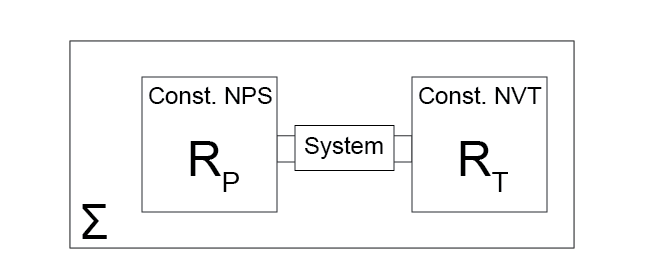
Connecting the system to the work reservoir allows it to be held at constant pressure since the system will exchange volume with the work reservoir to maintain a constant pressure when the system is at equilibrium (we have not yet proven that this occurs, but will do so in a future lecture). We assume that the connection to each reservoir is controllable (i.e. interactions can be turned on or off), the thermal reservoir is held at constant \(\underline{V}\) and \(N\), the work reservoir is held at constant \(\underline{S}\) and \(N\), and that changes to one reservoir do not affect the other.

Finally, we place the entire connected system in isolation, such that if we consider the system and both reservoirs the total entropy, volume, and number of particles is fixed. Referring to the global system as \(\Sigma\), we thus hold the system at constant \(\underline{S}^\Sigma, \underline{V}^\Sigma, N^\Sigma\). We allow the system to come to a global equilibrium, and then consider the effect of small perturbations from this equilibrium as we did previously in determining the condition of equilibrium for the energy and entropy.

Two lectures ago, we concluded that any perturbations to a system at equilibrium that is held at constant entropy necessarily increases the internal energy. We can thus write for the total isolated system:

\[\Delta\underline{U}^\Sigma = \Delta\underline{U} + \Delta\underline{U}^{R_T} + \Delta\underline{U}^{R_P} > 0\]

where \(\underline{U}\) is the energy of the system, \(\underline{U}^{R_T}\) is the energy of the thermal reservoir, and \(\underline{U}^{R_P}\) is the energy of the work reservoir. The entropy of the global system is constant and the work reservoir has adiabatic walls, but heat can exchange between the system and thermal reservoir so the entropy in these two systems can change. We can also write:

\[\begin{split}\begin{aligned} \Delta\underline{S}^\Sigma &= \Delta \underline{S} + \Delta\underline{S}^{R_T} = 0 \\ \Delta \underline{S}^{R_P} &= 0 \end{aligned}\end{split}\]

Similarly, the volume of the thermal reservoir is fixed, the volume of the global system is fixed, but the system under study can exchange volume with the work reservoir:

\[\begin{split}\begin{aligned} \Delta\underline{V}^\Sigma &= \Delta \underline{V} + \Delta\underline{V}^{R_P} = 0 \\ \Delta \underline{V}^{R_T} &= 0 \end{aligned}\end{split}\]

Finally, the number of particles is fixed in each subsystem:

\[\Delta N^\Sigma = \Delta N = \Delta N^{R_T} = \Delta N^{R_P} = 0\]

Now we can consider variations of the system that allow us to consider the behavior of different thermodynamic potentials.

Case 1: When there are interactions with the work reservoir and no interactions with the thermal reservoir, show that the enthalpy \(H\) is minimized at equilibrium.

Click for answer

In this case, we assume that the thermal reservoir is not part of the system so that \(\Delta \underline{S}^{R_T} = 0\) and thus \(\Delta \underline{S} = 0\). However, the pressure is kept constant due to contact with the work reservoir; the system is at constant \(\underline{S}\), \(P\), and \(N\). Now, we consider a perturbation to the system such that \(\Delta \underline{U}^{\Sigma} > 0\).

First, we write the energy change of the work reservoir using the first law as:

\[\Delta \underline{U}^{R_P} = -P \Delta \underline{V}^{R_P}\]

From the volume constraint (\(\underline{V}^{R_P}=-\underline{V}\)), this is equivalent to:

\[\Delta \underline{U}^{R_P} = P\Delta\underline{V}\]

Substituting into the system energy, with \(\Delta \underline{U}^{R_T} = 0\) since there is no work interaction with the thermal reservoir, we get:

\[\begin{split}\begin{aligned} \Delta \underline{U}^{\Sigma} &= \Delta \underline{U} + \Delta\underline{U}^{R_T} + \Delta\underline{U}^{R_P} > 0 \\ &= \Delta \underline{U} + P\Delta \underline{V} > 0 \\ \therefore \Delta \underline{H} &> 0 \end{aligned}\end{split}\]

Here, \(H\) is the enthalpy of the enthalpy, which we can see is a Legendre transform of the energy (\(H = U + PV\)). Therefore, any change in the system held at constant \(\underline{S}, \underline{P}, N\) increases the enthalpy; the enthalpy is minimized for a system with constant \(\underline{S}, \underline{P}, N\) at equilibrium.

Case 2: When there is no interaction with the work reservoir and interactions with the thermal reservoir, show that the Helmholtz free energy \(F\) is minimized at equilibrium.

Click for answer

Similar idea as above. The system of interest is now held at constant \(\underline{V}, T, N\) since interactions with the work reservoir are not allowed, but heat can be exchanged with the thermal reservoir to maintain constant temperature. Following the same logic as above, we can use the first law (with \(\Delta \underline{V}^{R_T} = 0\)) to write:

\[\begin{aligned} \Delta \underline{U}^{R_T} &= T \Delta \underline{S}^{R_T} = -T\Delta\underline{S} \end{aligned}\]

Substituting into the change in energy of the global system (with again \(\Delta \underline{U}^{R_P} = 0\) since there is no interaction with the work reservoir) yields:

\[\begin{split}\begin{aligned} \Delta \underline{U}^{\Sigma} &= \Delta \underline{U} + \Delta\underline{U}^{R_T} + \Delta\underline{U}^{R_P} > 0 \\ &= \Delta \underline{U} - T\Delta \underline{S} \\ \therefore \Delta \underline{F} > 0 \end{aligned}\end{split}\]

Hence, the Helmholtz free energy is minimized for a system with constant \(T, \underline{V}, N\) at equilibrium.

Case 3: When there are interactions with both the work reservoir and thermal reservoir, show that the Gibbs free energy \(G\) is minimized at equilibrium.

Click for answer

Finally, we consider a case in which both reservoirs interact with the system, so the system is at constant \(T, P, N\). We can combine the logic from the two cases above to write:

\[\begin{split}\begin{aligned} \Delta \underline{U}^{R_P} &= P\Delta\underline{V} \\ \Delta \underline{U}^{R_T} &= -T\Delta\underline{S} \\ \Delta \underline{U}^{\Sigma} &= \Delta \underline{U} + \Delta \underline{U}^{R_T} + \Delta \underline{U}^{R_P} > 0 \\ &= \Delta \underline{U} - T\Delta \underline{S} + P\Delta\underline{V} \\ \therefore \Delta \underline{G} > 0 \end{aligned}\end{split}\]

The Gibbs free energy is minimized for a system with constant \(T, P, N\) at equilibrium.

Relationship between partial derivatives

The introduction of new thermodynamic potentials gives rise to a series of new partial derivatives that tend to appear in thermodynamic relationships.

Remember, we can relate known thermodynamic variables to the exact differentials of thermodynamic potentials with respect to their natural variables. In other cases, we might also define an exact differential of a thermodynamic potential in terms of arbitrary parameters that are not the natural variables of the potential, in which case we need methods to relate partial derivatives to measurable quantities. Here, we briefly review several rules for helping simplify partial derivatives, as this will be an important aspect of solving problems when confronted with derivatives that are not easily measurable experimentally.

Inversion of derivatives

\[\left ( \frac{\partial f}{\partial y}\right )_x = \left ( \frac{\partial y}{\partial f}\right )_x^{-1}\]

For example: \(\left ( \frac{\partial S}{\partial P}\right )_T = \left ( \frac{\partial P}{\partial S}\right )_T^{-1}\)

Triple product rule

\[\left ( \frac{\partial f}{\partial x}\right )_y \left ( \frac{\partial x}{\partial y}\right )_f \left ( \frac{\partial y}{\partial f}\right )_x = -1\]

For example: \(\left ( \frac{\partial H}{\partial T}\right )_P \left ( \frac{\partial T}{\partial P}\right )_H \left ( \frac{\partial P}{\partial H}\right )_T = -1\)

Chain rule to add another variable

\[\left ( \frac{\partial f}{\partial y}\right )_x = \frac{(\partial f / \partial z )_x}{(\partial y / \partial z )_x} = \left ( \frac{\partial f}{\partial z}\right )_x \left ( \frac{\partial z}{\partial y}\right )_x\]

For example: \(\left ( \frac{\partial S}{\partial H}\right )_P = \frac{(\partial S / \partial T )_P}{(\partial H / \partial T )_P} = \frac{C_P/T}{C_P} = \frac{1}{T}\)

The expansion rule

This rule is a bit less obvious than the others. We will provide an example here, and proof of this rule is provided in the appendices:

\[\begin{aligned} \left ( \frac{\partial f}{\partial u}\right )_{v} &= \left ( \frac{\partial f}{\partial x}\right )_{y} \left ( \frac{\partial x}{\partial u}\right )_{v} + \left ( \frac{\partial f}{\partial y}\right )_{x} \left ( \frac{\partial y}{\partial u}\right )_{v} \end{aligned}\]

This rule is most commonly used when initially given a total derivative. For example:

\[\begin{split}\begin{aligned} dS &= \left ( \frac{\partial S}{\partial T} \right )_V dT + \left ( \frac{\partial S}{\partial V} \right )_T dV \\ \therefore \left ( \frac{\partial S}{\partial T} \right )_P &= \left ( \frac{\partial S}{\partial T} \right )_V \left ( \frac{\partial T}{\partial T} \right )_P + \left ( \frac{\partial S}{\partial V} \right )_T \left ( \frac{\partial V}{\partial T} \right )_P \\ &= \left ( \frac{\partial S}{\partial T} \right )_V + \left ( \frac{\partial S}{\partial V} \right )_T \left ( \frac{\partial V}{\partial T} \right )_P \end{aligned}\end{split}\]

In this example, it may look like I differentiated both sides of the total derivative of \(S\), but if that were so I would need to include extra terms due to the product rule. What I have actually done is employ the expansion rule with \(f=S\), \(x=T\), \(y=V\), \(u=T\), and \(v=P\). Setting \(x=u\) removes one of the derivatives from the expression.

Maxwell reciprocity

\[\begin{split}\begin{aligned} \left ( \frac{\partial(\partial f / \partial y )_x}{\partial x} \right )_y &= \left ( \frac{\partial(\partial f / \partial x )_y}{\partial y} \right )_x \\ f_{yx} &= f_{xy} \end{aligned}\end{split}\]

The second line illustrates alternative notation that we may use on occasion; the key point is that mixed second derivatives are equivalent regardless of the order of differentiation.

Partial derivatives in thermodynamics

Maxwell relations

This last relation - Maxwell reciprocity - will pop up repeatedly by establishing the notion of a

Maxwell relation

equivalence in thermodynamic second derivatives established by Maxwell reciprocity

We will present an example of a Maxwell relation now, and later show how this procedure can be generalized. First, consider an expression for the Gibbs free energy in differential form:

\[\begin{split}\begin{aligned} dG &= -S dT + V dP \\ &= \left ( \frac{\partial G}{\partial T}\right )_{P} dT + \left ( \frac{\partial G}{\partial P}\right )_{T} dP \end{aligned}\end{split}\]

We can now take derivatives of \(-S\) and \(V\) with respect to \(P\) and \(T\) respectively, which are equivalent according to the Maxwell reciprocity theorem:

\[\begin{split}\begin{aligned} -S &= \left ( \frac{\partial G}{\partial T}\right )_{P} \\ V &= \left ( \frac{\partial G}{\partial P}\right )_{T} \\ \left ( \frac{\partial (\partial G/\partial T)_P}{\partial P}\right )_{T} &= \left ( \frac{\partial (\partial G/\partial P)_T}{\partial T}\right )_{P} \\ \therefore -\left ( \frac{\partial S}{\partial P}\right )_{T} &= \left ( \frac{\partial V}{\partial T}\right )_{P} \end{aligned}\end{split}\]

Maxwell relations thus relate second derivatives of the fundamental relation to each other, which is often very useful for transforming derivatives into forms that are related to materials properties will be demonstrated in the Problem Sets.

Shameless plug: if you want to see Maxwell relations in action, check out Prof. Cersonsky’s first paper.

Behavior of state functions

Finally, let’s remind ourselves of relationships assocated with state functions, although we have already been performing these manipulations. We define \(B\) as a state function (i.e., a derived or primative property of a system, including the energy, thermodynamic parameters, mechanical properties, or any parameters discussed to date excluding heat and work). We can write \(B\) as a function of three independently variable parameters, \(x\), \(y\), and \(z\), as:

\[\begin{aligned} B = f(x,y,z) \end{aligned}\]

Note that in the past we have largely assumed that \(x\), \(y\), and \(z\) are the natural variables when \(B\) is a thermodynamic potential (i.e., the energy, entropy, or a free energy), but this is not necessary. The difference in the value of \(B\) can always be written as the difference in \(f(x,y,z)\) for any two stable equilibrium states:

\[\begin{aligned} \Delta B = B_2 - B_1 = f(x_2, y_2, z_2) - f(x_1, y_1, z_1) \end{aligned}\]

We can also write \(B\) in differential form as an exact differential as a function of \(x\), \(y\), and \(z\):

\[\begin{aligned} dB &= \left ( \frac{\partial f}{\partial x}\right)_{y, z} dx + \left ( \frac{\partial f}{\partial y}\right)_{x, z} dy + \left ( \frac{\partial f}{\partial z}\right)_{x, y} dz \end{aligned}\]

We can then compute the change \(\Delta B\) along a specified path by integrating this exact differential. The path will stipulate the limits of integration for each variable as well as the values that are fixed. However, the actual path chosen does not affect the value of \(\Delta B\) since it is a state function, so we can integrate along any convenient path. For example, we could calculate the change in \(B\) from state 1 to state 2 in which we proceed to \(x_2\) along a constant \(y_1, z_1\) path, to \(y_2\) along a constant \(x_2, z_1\) path, then to \(z_2\) along a constant \(x_2, y_2\) path. The corresponding integral is then:

\[\begin{aligned} \Delta B &= \int_{x_1}^{x_2} \left ( \frac{\partial f}{\partial x}\right)_{y_1, z_1} dx + \int_{y_1}^{y_2} \left ( \frac{\partial f}{\partial y}\right)_{x_2, z_1} dy + \int_{z_1}^{z_2} \left ( \frac{\partial f}{\partial z}\right)_{x_2, y_2} dz \end{aligned}\]

Note that we have to be careful about what variables are held constant, or more specifically where in the overall phase space each of these derivatives is evaluated.

Euler’s Theorem

We will now introduce Euler’s Theorem, which will be useful for interpreting the fundamental relation.

Euler’s theorem

if a function \(f(a,b,x,y)\) obeys the relation:

\[f(a, b, Kx, Ky) = K^hf(a, b, x, y),\]

where \(K\) and \(h\) are constants, then

(33)\[x \frac{\partial}{\partial x}[ f(a, b, x, y)] + y \frac{\partial}{\partial y} [f(a, b, x, y) ] = h f(a, b, x, y)\]

We describe \(f(a,b,x,y)\) as homogeneous to degree \(h\) in \(x\) and \(y\). We can see from this definition that \(a\) and \(b\) correspond to intensive variables and \(x\) and \(y\) to extensive variables using our thermodynamics nomenclature, in that multiplying \(x\) and \(y\) by a constant (i.e. the amount of material) changes the value of the function by the same constant without needing to change the values of \(a\) and \(b\). While we have written this expression in terms of four variables, it can be generalized to any number of them.

We can apply this relation to the fundamental relation (we will use the energy representation) by recognizing that the fundamental relation is homogeneous to degree 1 (\(h=1\)) with respect to extensive variables. We can then write:

\[\underline{U}(K\underline{S}, K\underline{V}, KN) = K\underline{U}(\underline{S}, \underline{V}, N)\]

This relation is apparent because each of the variables is extensive, so multiplying all of them by \(K\) is equivalent to multiplying the energy by \(K\). Comparing to (33), we have \(x = \underline{S}\), \(y = \underline{V}\), and a third extensive variable \(z = N\). We can write a generalized version of (33) for this system:

(34)\[\begin{split}\begin{aligned} &x \frac{\partial}{\partial x}[ f(x,y,z)] + y \frac{\partial}{\partial y} [f(x,y,z) ] + z \frac{\partial}{\partial z} [f(x,y,z) ] = \nonumber \\ & \underline{S} \left ( \frac{\partial \underline{U}(\underline{S}, \underline{V}, N)}{\partial \underline{S}} \right )_{\underline{V}, N} + \underline{V} \left ( \frac{\partial \underline{U}(\underline{S}, \underline{V}, N)}{\partial \underline{V}} \right )_{\underline{S}, N} + N \left ( \frac{\partial \underline{U}(\underline{S}, \underline{V}, N)}{\partial N} \right )_{\underline{S}, \underline{V}} \\ &= \underline{S}T - \underline{V} P + N \mu = hf(x, y, z) \\ &\therefore \underline{U}(\underline{S}, \underline{V}, N) = T\underline{S} - P\underline{V} + N\mu \end{aligned}\end{split}\]

This is a useful expression for the energy; we can also derive another useful relation by taking the total differential of (34):

\[\begin{aligned} d\underline{U} = Td\underline{S} + \underline{S} dT - Pd\underline{V} - \underline{V}dP + Nd\mu + \mu dN \end{aligned}\]

We can compare this with the combined first and second law for an open system:

\[\begin{aligned} d\underline{U} = Td\underline{S} - Pd\underline{V} + \mu dN \end{aligned}\]

Equating these expressions leads to the

Gibbs-Duhem equation

\[\underline{S}dT - \underline{V}dP + Nd\mu = 0\]

The Gibbs-Duhem equation will be used extensively in our study of multiphase systems in a generalized form. The importance of this relation is that it places a constraint on \(T\), \(P\), and \(\mu\) such that they cannot all be independently variable; indeed, in general if we have a multicomponent system with \(n+2\) (always) intensive variables, we can also express any one intensive variable in terms of the other \(n+1\) intensive variables using this relation.

Show that the enthalpy \(H = T\underline{S} + \mu N\).

Click for answer

First, we define the enthalpy as:

\[\begin{split}\begin{aligned} d\underline{H} &= Td\underline{S} + \underline{V} dP + \mu dN \\ \underline{H} &= \underline{H}(\underline{S}, P, N)\\ \underline{H}(K\underline{S}, P, KN) &= K\underline{H}(\underline{S}, P, N) \end{aligned}\end{split}\]

For the enthalpy, since \(P\) is an intensive variable, multiplying it by a factor of \(K\) leaves it unchanged; therefore we associate \(a = P\), \(x = \underline{S}\), and \(y=N\) to get from (33):

\[\begin{split}\begin{aligned} hf(a, x, y) &= x \frac{\partial}{\partial x}[ f(a, x, y)] + y \frac{\partial}{\partial y} [f(a, x, y) ] \\ \underline{H} &= \left ( \frac{\partial \underline{H}}{\partial{S}}\right )_{P, N} \underline{S} + \left ( \frac{\partial \underline{H}}{\partial{N}}\right )_{P, \underline{S}} N \\ &= T\underline{S} + \mu N \end{aligned}\end{split}\]

Show that the Gibbs free energy \(G = \mu N\).

Click for answer

As a last example, we consider the Gibbs free energy:

\[\begin{split}\begin{aligned} d\underline{G} &= -\underline{S} dT + \underline{V} dP + \mu dN \\ \underline{G} &= \underline{G}(T, P, N)\\ \underline{G}(T, P, KN) &= K\underline{G}(T, P, N) \end{aligned}\end{split}\]

Here, \(a=T\), \(b=P\), and \(x=N\), leading to:

\[\begin{split}\begin{aligned} hf(a, b, x) &= x\frac{\partial}{\partial x}[ f(a, b, x)] \\ \underline{G} &= \left ( \frac{\partial \underline{G}}{\partial{N}}\right )_{T, P} N \\ &= \mu N \end{aligned}\end{split}\]

This last equation is a useful one that we will return to in later lectures. Note that we could obtain the same expression by performing a Legendre transform of the internal energy to obtain \(\underline{G} = U - T\underline{S} + P\underline{V}\) and substituting in the Euler integrated form of the internal energy, thus showing consistency between our different derivations.

These expressions can all be generalized for other combinations of intensive and extensive variables accordingly.

Link to Shared Notes