Equilibrium in single-component systems

Additional Readings for the Enthusiast

Tester and Modell [4], Ch. 6.2, 6.4, 7.1, 7.2, 8.1-8.3

Goals for Today’s Lecture

• What behavior would we expect from intensive variables at equilibrium?

• What are the criteria for phase coexistence?

• When will a single phase system undergo a first-order phase transition?

• How does differential scanning calorimetry work?

Equilibrium conditions

For simple, single-component systems at equilibrium, certain thermodynamic potentials are either minimized or maximized depending on the parameters held constant in that system. We will now expand upon the concept that a system at equilibrium is stable with respect to variations, then apply this framework to study conditions of equilibrium in multicomponent systems.

If our system is at stable equilibrium, any changes will ______ the entropy.

decrease

Correct! Entropy is maximized at equilibrium, so changes will decrease the entropy.

increase

Whoops, try again!

We can determine if a given system is at equilibrium by its response to a small variation in thermodynamic parameters. Testing such “virtual” variations was effectively the procedure used in the preceding lecture to illustrate how other thermodynamic potentials respond at equilibrium. Here, we will formalize the notation for analyzing the response of a system to small variations; later, we will consider stability with respect to very large variations in system parameters.

Consider an isolated system. We will write an expression for the effect of a small perturbation with respect to a parameter \(z_i\) on the entropy, \(\delta \underline{S}\), recognizing that the perturbation is small. Recall from our earlier lecture that we mentioned that there are \(n+2\) independently variable parameters (i.e. \(\underline{U}\),\(\underline{V}\), \(N_1\), etc.). We will now consider calculating the change in the entropy, \(\Delta \underline{S}\), associated with a series of small perturbations \(\delta z_i\), where \(z_i\) refers to one of the \(n+2\) independently variable parameters; if all the \(\delta z_i\) are sufficiently small, we can calculate the change in entropy by Taylor expanding around the original value of \(S\):

\[\Delta \underline{S} = \delta \underline{S} + \frac{1}{2!} \delta^2 \underline{S} + \frac{1}{3!} \delta^3 \underline{S} \dots \]

where

\[\delta \underline{S} = \sum_{i=1}^{n+2} \left ( \frac{\partial \underline{S}}{\partial z_i} \right ) \delta z_i \equiv \sum_{i=1}^{n+2} \underline{S}_{z_i} \delta z_i\]

and

\[\delta^2 \underline{S} = \sum_{i=1}^{n+2} \sum_{j=1}^{n+2} \left ( \frac{\partial^2 \underline{S}}{\partial z_i\partial z_j} \right ) \delta z_i \delta z_j \equiv\sum_{i=1}^{n+2} \sum_{j=1}^{n+2} \underline{S}_{z_i z_j} \delta z_i \delta z_j\]

We can continue this framework for higher order derivatives. Here, note the notation we use, as adopted from the section on Maxwell reciprocity - the subscripts on \(\underline{S}\) indicates partial derivative(s) with respect to the subscripted variable.

At equilibrium, we have now established two conditions that must be true:

\[\begin{split}\begin{aligned} \delta \underline{S} &= 0 \\ \delta^2 \underline{S} &< 0 \end{aligned}\end{split}\]

If I were to plot \(\underline{S}\) with respect to all possible \(z_i\), the first condition indicates that there is an extremum in \(\underline{S}\), while the second condition ensures that it is a maximum, and thus small perturbations to the system will decrease the entropy.

Phase equilibrium in multi-component systems

Let us now consider the conditions of equilibrium for a multiphase system; that is, a complex system which can be divided into multiple simple subsystems representing multiple phases. Each phase has its own unique properties, but all phases consist of the same components.

For example:

• the liquid state of a molecule is in equilibrium with the vapor phase of the same molecule; in this case the two phases correspond to different states of aggregation and are distinguished by different densities

• a mixture of oil and water that separates into two liquid phases, one of which is primarily oil and the other of which is primarily water; the compositions of each phase are distinct but again the same components exist in each phase.

In general, it will be hard to identify physical “boundaries” to each phase in a multiphase system; however, we can construct virtual walls that divides a complex isolated system into multiple subsystems, each of which represents a different phase.

We will now derive constraints placed on intensive variables of a multiphase system. Let us consider a general case where a system has two phases, \((1)\) and \((2)\), and two components, \(A\) and \(B\). We can imagine an isolated, complex system that is divided into two simple subsystems, each corresponding to a phase.

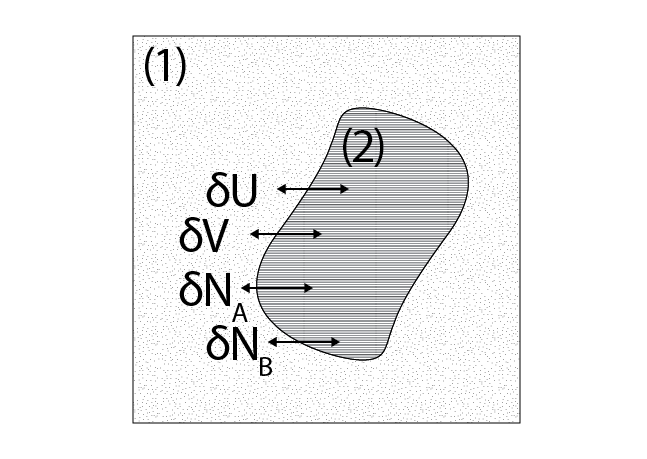
Our subsystems are connected such that they can exchange heat (and therefore \(\underline{U}\)), volume, and material, such that the system is subject to the following constraints at equilibrium:

\[\begin{split}\begin{aligned} \delta \underline{S} &= \delta \underline{S}^{(1)} + \delta \underline{S}^{(2)} = 0\\ \delta \underline{U} &= \delta \underline{U}^{(1)} + \delta \underline{U}^{(2)} = 0\\ \delta \underline{V} &= \delta \underline{V}^{(1)} + \delta \underline{V}^{(2)} = 0 \\ \delta {N_A} &= \delta N_A^{(1)} + \delta N_A^{(2)} =0 \\ \delta {N_B} &= \delta N_B^{(1)} + \delta N_B^{(2)} =0 \end{aligned}\end{split}\]

Each of these thermodynamic parameters has a corresponding conjugate variable associated with its individual phase (e.g. \(T^{(1)}\) and \(T^{(2)}\)). The first constraint is from the condition that the entropy reaches an extremum at equilibrium as discussed above, while the rest are due to the boundaries of the isolated system. Using the entropy representation of the fundamental relation, we can then write:

\[\begin{split}\begin{aligned} \delta \underline{S} &= \delta \underline{S}^{(1)} + \delta \underline{S}^{(2)} \\ &= \sum_{i=1}^{n+2} \underline{S}^{(1)}_{z_i} \delta z_i + \sum_{i=1}^{n+2} \underline{S}^{(2)}_{z_i} \delta z_i \\ &= \frac{1}{T^{(1)}} \delta \underline{U}^{(1)} + \frac{1}{T^{(2)}} \delta \underline{U}^{(2)} + \frac{P^{(1)}}{T^{(1)}} \delta \underline{V}^{(1)} + \frac{P^{(2)}}{T^{(2)}} \delta \underline{V}^{(2)} - \nonumber \\ &\frac{\mu_A^{(1)}}{T^{(1)}} \delta N_A^{(1)} - \frac{\mu_A^{(2)}}{T^{(2)}} \delta N_A^{(2)} - \frac{\mu_B^{(1)}}{T^{(1)}} \delta N_B^{(1)} - \frac{\mu_B^{(2)}}{T^{(2)}} \delta N_B^{(2)} = 0 \end{aligned}\end{split}\]

The important part here is that the variation in the entropy must be zero with respect to all possible variations - that is, for any variation in any other parameter. Substituting in the constraints above gives:

\[\begin{split}\begin{aligned} \delta \underline{S} = & \left (\frac{1}{T^{(1)}} - \frac{1}{T^{(2)}} \right ) \delta \underline{U}^{(1)} + \left ( \frac{P^{(1)}}{T^{(1)}} - \frac{P^{(2)}}{T^{(2)}}\right )\delta \underline{V}^{(1)} \\ & - \left ( \frac{\mu_A^{(1)}}{T^{(1)}} - \frac{\mu_A^{(2)}}{T^{(2)}} \right ) \delta N_A^{(1)} - \left ( \frac{\mu_B^{(1)}}{T^{(1)}} - \frac{\mu_B^{(2)}}{T^{(2)}} \right ) \delta N_B^{(1)} = 0 \end{aligned}\end{split}\]

In the most general case, there is no constraint on the value of \(\delta \underline{U}^{(1)}\) or the variation of any other parameter associated with the individual simple systems. If there are multiple non-zero parameters that vary, then the condition that \(\delta \underline{S} = 0\) for the isolated, combined system can only be satisfied for all possible variations in the parameters if each prefactor on the varying parameter is zero. This means that equilibrium is satisfied only if:

\[\begin{split}\begin{aligned} T^{(1)} &= T^{(2)} \label{equal_temp}\\ P^{(1)} &= P^{(2)} \label{equal_pres}\\ \mu_A^{(1)} &= \mu_A^{(2)} \\ \mu_B^{(1)} &= \mu_B^{(2)} \end{aligned}\end{split}\]

This assumes that the virtual boundary between the two systems is diathermal (\(\delta \underline{U}^{(1)} \ne 0\)), movable (\(\delta \underline{V}^{(1)} \ne 0\)), and permeable to both components (\(\delta N_A^{(1)} \ne 0\) and \(\delta N_B^{(1)} \ne 0\)).

How would these conditions change if the wall was rigid?

Click for answer

If the wall is rigid, then \(\delta \underline{V}^{(1)} = \delta \underline{V}^{(2)} = 0\), so substituting this expression into the above logic indicates that there would no longer be any condition on the equivalence of the pressure of the two subsystems, although all other conditions would be met.

Therefore, from this analysis we derive the following general rule: if two systems are able to exchange the extensive parameter \(X\), then at equilibrium the conjugate intensive parameter \(f\) (a first derivative of the fundamental relation) will be equal between the two systems. These conditions are equally applicable to phases within a single system or to the interactions between a system and a reservoir.

Phase equilibrium in single-component systems

When we will observe a single-phase system?

First, let’s choose an ensemble with which to understand this problem. Consider a single-component system placed in a container with movable boundaries at constant temperature, like a sample in a beaker, where the beaker is open to air, allowing the sample to change its volume. This setup, which is common for many laboratory conditions, exists naturally in the isobaric-isothermal ensemble, for which the natural variables are \(N\), \(P\), and \(T\), and our thermodynamic potential is the Gibbs free energy.

In the last lecture, we used Euler’s theorem to relate the Gibbs free energy to the chemical potential via the relation:

\[\begin{split}\begin{aligned} \underline{G} &= \left ( \frac{\partial \underline{G}}{\partial{N}}\right )_{T, P} N \\ &= \mu N \end{aligned}\end{split}\]

Let’s now consider a system which can form two possible phases, denoted by \((1)\) and \((2)\), with corresponding chemical potentials \(\mu^{(1)}\) and \(\mu^{(2)}\). Since we have established that at equilibrium the Gibbs free energy of the system will be minimized, the Euler integrated expression for the Gibbs free energy provides a straightforward relationship to determine which phase will be observed. Namely, at equilibrium in a single-component system at constant \(T\) and \(P\):

\[\begin{aligned} \underline{G} &= \mu^{(1)}N^{(1)} + \mu^{(2)}N^{(2)} \end{aligned}\]

Recognizing that \(\underline{G}\) is minimized at equilibrium, and that the amount of material can freely exchange between the two phases:

Which phase is observed when \(\mu^{(1)} < \mu^{(2)}\)?

Click for answer

Phase (1).

Which phase is observed when \(\mu^{(1)} > \mu^{(2)}\)?

Click for answer

Phase (2).

Which phase is observed when \(\mu^{(1)} = \mu^{(2)}\)?

Click for answer

Both phases.

Note that this is fully consistent with our conditions of equilibrium described above.

We thus see that the chemical potential emerges as the most important quantity for determining phase behavior, but in principle we cannot control this as easily as the temperature and pressure. However, recall that the Gibbs-Duhem equation from last lecture places a constraint on the \(n+2\) intensive variables of a thermodynamic potential such that only \(n+1\) are independently variable. For a single component system, the Gibbs-Duhem equation states:

\[\begin{split}\begin{aligned} N d\mu &= -\underline{S} dT + \underline{V} dP \\ d\mu &= - SdT + VdP \\ \therefore \mu &= f_1(T,P) \end{aligned}\end{split}\]

where \(f_1\) is some function that is unknown and system specific. We can now further write a more general expression for \(\mu\) in terms of experimentally measurable quantities by expressing \(S\) and \(V\) as functions of \(T\) and \(P\) and integrating relative to a reference state:

\[\begin{aligned} \mu = \mu^0 - \int_{T^0}^T [S(T, P)]_{P^0} dT + \int_{P^0}^P [V(T, P)]_{T} dP \end{aligned}\]

Note that here we perform the integration by first integrating along an isobaric path at the reference state pressure, \(P^0\), then integrating along an isothermal path at the temperature of interest, \(T\). \(\mu^0\) is the reference state chemical potential. We can now further write out expressions for \(S(T,P)\) and \(V(T, P)\) by integrating their exact differentials:

\[\begin{split}\begin{aligned} dS &= \left ( \frac{\partial S}{\partial T} \right )_{P} dT + \left ( \frac{\partial S}{\partial P} \right )_{T} dP \\ dV &= \left ( \frac{\partial V}{\partial T} \right )_{P} dT + \left ( \frac{\partial V}{\partial P} \right )_{T} dP \end{aligned}\end{split}\]

Fortunately, these partial derivatives can be simplified by recognizing the definitions of three experimentally measurable materials parameters, which you have encountered on Problem Set 5:

\[\begin{split}\begin{aligned} C_P &\equiv T \left ( \frac{\partial S}{\partial T} \right )_P \quad \text{Heat capacity at constant pressure} \\ \alpha &\equiv \frac{1}{V} \left ( \frac{\partial V}{\partial T} \right )_P \quad \text{Coefficient of thermal expansion} \\ \beta &\equiv -\frac{1}{V} \left ( \frac{\partial V}{\partial P} \right )_T \quad \text{isothermal compressibility} \end{aligned}\end{split}\]

Substituting these expressions into the exact differentials above, and recognizing the Maxwell relation \(\left ( \frac{\partial S}{\partial P} \right )_{T} = -\left ( \frac{\partial V}{\partial T} \right )_{P}\), gives:

\[\begin{split}\begin{aligned} dS &= \frac{C_P}{T} dT - \alpha V dP \\ dV &= \alpha V dT - \beta V dP \end{aligned}\end{split}\]

All prefactors are now experimentally measurable system-specific parameters. Integrating each of these expressions from a reference state (again along an isobaric then isothermal path) and substituting into the prior expression for the chemical potential yields:

\[\begin{split}\begin{aligned} S &= S^0 + \int_{T^0}^T \left [\frac{C_P}{T} \right ]_{P^0} dT - \int_{P^0}^P [\alpha V]_{T} dP \\ V &= V^0 + \int_{T^0}^T [\alpha V]_{P^0} dT - \int_{P^0}^P [\beta V]_{T} dP \\ \mu &= \mu^0 - (T-T^0) S^0 + (P-P^0)V^0 \\ & - \int_{T^0}^T \left [ \int_{T^0}^T \left [\frac{C_P}{T} \right ]_{P^0} dT - \int_{P^0}^P [\alpha V]_{T} dP \right ]_{P^0} dT \nonumber \\ & + \int_{P^0}^P \left [ \int_{T^0}^T [\alpha V]_{P^0} dT - \int_{P^0}^P [\beta V]_{T} dP \right ]_{T} dP \nonumber \end{aligned}\end{split}\]

This expression is obviously quite complicated, with the only obvious simplification being the elimination of the term \(\int_{P^0}^P [\alpha V]_{T} dP\) because this integral is performed at constant \(P^0\) and thus the upper and lower limits of integration are the same. The key point, however, is that we have now reduced our expression for the chemical potential to be only a function of experimentally measurable parameters - that is, \(T\), \(P\), \(\alpha\), \(\beta\), and \(C_P\). We also have introduced parameters related to the reference state, as indicated by the superscript \(0\), but in general we can choose arbitrary values of \(S^0\) and \(\mu^0\) and need only know the physical values of \(P^0\), \(V^0\), and \(T^0\) for a reference state of interest.

Phase behavior in single-component systems - PVT Diagrams

The expression for the chemical potential presented above is fully defined if we know the materials parameters \(\alpha\), \(\beta\), \(C_P\), their temperature and pressure variations, and the pressure, volume, and temperature of a reference state. However, since \(\alpha\) and \(\beta\) themselves are defined in terms of the variation of the volume with respect to temperature and pressure, it is also equally reasonable to specify the behavior of \(C_P\) and the relationship between the pressure, volume, and temperature.

In other words, if we know the behavior of a system across PVT we can fully specify its phase behavior because PVT behavior defines all parameters that appear in the expression for the chemical potential. The approach of specifying PVT behavior is much more prominent in the literature than specifying \(\alpha\) and \(\beta\).

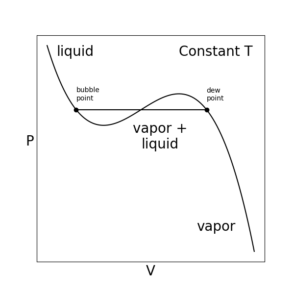
We can visualize PVT behavior by plotting constant-temperature isotherms as a function of volume.

Some observations:

• Repeating these measurements for a series of temperatures would yield the \(PVT\) equation of state for the system, which reflects the fundamental equation for the system.

• The behavior in this plot is typical of behavior described by a cubic equation of state, such as the well-known van der Waals equation of state.

dew point

the volume of the system where liquid starts to precipitate from the vapor phase

vapor pressure

The pressure at which the vapor phase is in equilibrium with the liquid phase.

saturation pressure

Another name for the vapor pressure.

We can interpret this isotherm in terms of phase behavior:

1. If we were to prepare a system that is initially at equilibrium at a large value of \(V\), we would find that it is in a vapor phase.

2. If we then connect the system to a thermal reservoir at a fixed temperature and a volume reservoir with a controllable pressure, and imagine slowly increasing the pressure (or equivalently compressing the volume) at an infinitely slow rate (such that the system is always at equilibrium), we would find that the system would maintain a vapor state with a volume specified by the PVT isotherm until a small amount of liquid forms at the dew point.

3. As you continue to try to increase the pressure, you would observe more vapor phase condense to the liquid phase without the pressure changing until eventually the entire system is liquid, which occurs at the vapor pressure or the saturation pressure.

Following from the discussion above, at this pressure and temperature the chemical potential of a molecule in the low-molar-volume liquid phase is equal to the chemical potential of a molecule in the high-molar-volume vapor phase.

first-order phase transition

a transition in which a first derivative of a thermodynamic potential with respect to some thermodynamic parameter is discontinuous

The transition from a vapor phase with a well-defined molar volume (or equivalently, density) to a liquid phase with a smaller molar volume is an example of a first-order phase transition. The volume is the first deriative of the Gibbs free energy with respect to pressure and the change in volume is discontinuous between the vapor and liquid states, satisfying this definition. Phase transitions between different states of aggregation all fit this criterion; the solid-liquid and solid-vapor transitions would also involve discontinuities in the volume.

First-order phase transitions are also distinguished by the relase or adsorption of latent heat during the transition. The latent heat is equal to the molar enthalpy difference, \(\Delta H\), between the two phases; since enthalpy is a state function, the enthalpy of a particular phase at a specific temperature and pressure is a material property that will differ between different phases, especially if the phases are different states of aggregation. Therefore, the transition between states of aggregation will either require the input or release of energy to account for these molar enthalpy differences (note that it is an enthalpy, not an energy, since the volumes of the states will generally be different as drawn above, requiring \(PV\) work to be done as well).

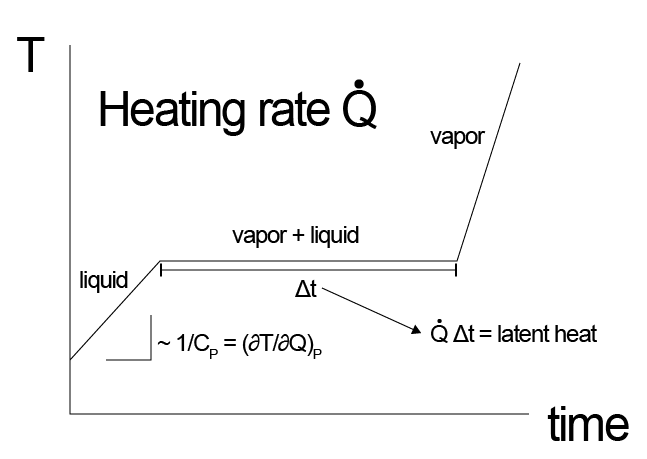
Importantly, the latent heat is enthalpy that is added to or removed from a system without the system temperature changing, since it accounts for the transformation of material from one state to another. Thus, if we were to imagine slowly heating up a solid until it melts to a liquid, we would observe that the temperature would first increase (at a rate given by the heat capacity of the material) and then would plateau at the melting point of the material while the phase transition is occurring, as all heat being adsorbed would be used for the conversion of solid to liquid. Once the phase transition is complete, the temperature would continue to rise at a different rate given the different heat capacity of the liquid phase.

During this process, we would have to change the rate of heat flow to maintain a constant change of temperature, which would allow us to determine the magnitude of the latent heat and heat capacities of both phases - this observation is the operating principle behind differential scanning calorimetry.

Link to Shared Notes