Ideal mixtures

Additional Readings for the Enthusiast

Tester and Modell [4], Ch. 9.5-9.7, 15.5

Goals for Today’s Lecture

• Define partial molar properties and give examples

• Define properties upon mixing and give examples

• Differentiate enthalpy and entropy of mixing and their positivity/negativity

• Define and compute the fugacity of mixing

• Define and describe ideal-gas mixtures and ideal solutions, and use them to simplify calculations of equilibrium conditions

Introduction to mixtures: partial molar properties

So far, we have only calculated the fugacity of a single-component system at phase equilibrium. Now, we will extend our framework to consider mixtures. First, let’s consider some simple definitions when dealing with mixtures. We define \(x_i\) as the mole fraction of component \(i\), such that:

\[\begin{split}\begin{aligned} x_i &\equiv \frac{N_i}{\sum_{i=1}^n N_i} \\ &= \frac{N_i}{N} \\ \sum_{i=1}^n x_i &= 1 \end{aligned}\end{split}\]

Each of the \(N_i\) is given in moles, and \(N\) is the total number of moles in the mixture. Note that by convention \(x_i\) refers to mole fractions in a liquid or solid phase and \(y_i\) refers to mole fractions in a vapor phase. Using \(x_i\) (or \(y_i\)) in place of \(N_i\) allows us to write an intensive form of some potential \(B\); for example, the intensive Gibbs free energy of a multicomponent mixture is then:

\[\begin{aligned} G(T,P,x_1, x_2, \dots x_n) \end{aligned}\]

We could also write two equivalent expressions for the extensive value of the Gibbs free energy:

\[\begin{aligned} \underline{G}(T,P, N_1, N_2,\dots N_n) = \underline{G}(T, P, x_1, x_2, \dots x_{n-1}, N) \end{aligned}\]

We can determine \(x_n\) from the other mole fractions by the constraint above. Now, let us consider what happens to system properties during the process of mixing relative to the properties of the independent pure components of that mixture. In other words, the process we consider is taking separate single-component systems and mixing their constituents into a single-phase mixture with a given composition.

For a mixture, why can’t we just compute the weighted average of the properties of the components? E.g. why, for volume, does \(V\ne x_1 V_1 + x_2 V_2\)?

Click for answer

The difference in volume will emerge from the interactions between the two components, which will likely differ in their attraction or repulsion from interactions of a given component with other molecules of the same type.

To account for interactions between components, we can instead define the increment in the value of some parameter \(B\) for the entire system upon addition of a single component, \(i\), we define the

partial molar property

of component \(i\), which is the increment in the value of some parameter \(B\) for the entire system upon addition of a single component, \(i\):

\[\begin{aligned} \overline{B}_i &\equiv \left(\frac{\partial \underline{B}}{\partial N_i}\right)_{T,P,N_j \ne N_i} \end{aligned}\]

Here, the overline indicates a partial molar property of component \(i\) and the partial derivative indicates the change in the (extensive) value of \(\underline{B}\) for the mixture upon increment of component \(i\), with the amount of each other component \(j\) held fixed. By definition, partial molar properties are defined with the temperature and pressure also held constant, as these are the two independent variables commonly associated with phase behavior.

Why are all partial molar properties intensive?

Click for answer

Because the derivative is always performed with respect to the number of moles of a single component.

We can define a simple expression for the extensive value of \(\underline{B}\) in terms of partial molar properties by again using Euler’s theorem. If we write the exact differential for \(\underline{B}\) as a function of the \(n\) components, \(T\), and \(P\), we obtain:

\[\begin{split}\begin{aligned} d\underline{B}(T,P, N_1, N_2, \dots, N_n) &= \left ( \frac{\partial \underline{B}}{\partial T}\right )_{P, N_j} dT + \left ( \frac{\partial \underline{B}}{\partial P}\right )_{T, N_j} dP + \sum_i^n \left ( \frac{\partial \underline{B}}{\partial N_i}\right )_{T,P, N_j \ne N_i} dN_i \\ &= \left ( \frac{\partial \underline{B}}{\partial T}\right )_{P, N_j} dT + \left ( \frac{\partial \underline{B}}{\partial P}\right )_{T, N_j} dP + \sum_i^n \overline{B}_i dN_i \end{aligned}\end{split}\]

By Euler’s theorem, we obtain expressions for the first-order derivative of \(\underline{B}\) with respect to each extensive variable (the set of \(N_i\)) multiplied by the corresponding extensive variable:

\[\begin{split}\begin{aligned} \underline{B} &= \sum_i^n \left ( \frac{\partial \underline{B}}{\partial N_i}\right )_{T,P, N_j \ne N_i} N_i \\ &= \sum_i^n \overline{B}_i N_i \end{aligned}\end{split}\]

Therefore, we obtain a straightforward expression for the extensive value of \(\underline{B}\) for a mixture in terms of partial molar properties of each component. Since \(\underline{B} = NB\), where \(N = \sum_i^n N_i\) is the total amount of material, we can also then obtain:

\[\begin{split}\begin{aligned} B &= \frac{\underline{B}}{N} \\ &= \frac{\sum_i^n \overline{B}_i N_i}{N} \\ &= \sum_i^n \overline{B}_i x_i \end{aligned}\end{split}\]

How is the chemical potential related to the partial molar Gibbs free energy?

Click for answer

They are equal!

If we let \(\underline{B} \equiv \underline{G}\), then the partial molar Gibbs free energy is given by:

\[\begin{aligned} \overline{G}_i &= \left ( \frac{\partial \underline{G}}{\partial N_i}\right )_{T,P, N_j \ne N_i} \end{aligned}\]

By comparison with the exact differential of the Gibbs free energy (defined in terms of its natural variables, such that it is a Legendre transform of the fundamental relation) we have:

\[\begin{split}\begin{aligned} d\underline{G} &= -\underline{S} dT + \underline{V} dP + \sum_i^n \mu_i dN_i \\ %&= \left ( \frac{\partial \underline{G}}{\partial T}\right )_{P, N_j} dT + \left ( \frac{\partial \underline{G}}{\partial P}\right )_{T, N_j} dP + \sum_i^n \left ( \frac{\partial \underline{G}}{\partial N_i}\right )_{T,P, N_{j, [i]}} dN_i \\ \therefore \mu_i &= \left ( \frac{\partial \underline{G}}{\partial N_i}\right )_{T,P, N_j \ne N_i} = \overline{G}_i \\ G &= \sum_i^n x_i \mu_i \end{aligned}\end{split}\]

We thus find that the partial molar Gibbs free energy of component \(i\) is identical to the chemical potential of component \(i\), and we regain an expression for the Gibbs free energy of the mixture that is similar to the expression for the Gibbs free energy of a single-component system that we obtained from Euler’s theorem.

Property changes upon mixing

We can now write the change in a given property upon mixing by considering the value of this property \(B\) of each of the \(n\) pure components and then the value of \(B\) for the mixture; since \(B\) is a state function, the pathway by which mixing occurs is irrelevant. We can thus write:

\[\begin{split}\begin{aligned} \Delta B_\textrm{mix} &= B - \sum_i^n x_i B_i \\ &= \sum_i^n x_i (\overline{B}_i - B_i) \end{aligned}\end{split}\]

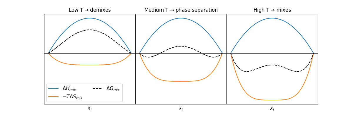
We call \(\Delta B_\textrm{mix}\) the change in the value of a property of a mixture relative to pure components the entropy of mixing, energy of mixing, free energy of mixing, etc. depending on \(B\). In this notation, \(B\) refers to the (intensive) value of \(B\) for the entire mixture while \(\sum_i^n x_i B_i\) is the value of \(B\) for each individual component weighted by the mole fraction of that component. Of particular interest is the Gibbs free energy of mixing; since the Gibbs free energy is minimized at equilibrium, mixing can only occur at equilibribum if \(\Delta G_\textrm{mix} < 0\) (although we will discuss that there is a subtlety here that may not be obvious). We can write for the Gibbs free energy of mixing:

\[\begin{aligned} \Delta G_\textrm{mix} &= \sum_i^n x_i (\overline{G}_i - G_i) \end{aligned}\]

We can break this free energy change into two separate components by recalling the definition of the Gibbs free energy from Euler’s theorem:

\[\begin{split}\begin{aligned} G &= U + PV - TS \\ &= H - TS \\ \therefore \Delta G_\textrm{mix} &= \Delta H_\textrm{mix} - T \Delta S_\textrm{mix} \end{aligned}\end{split}\]

Analysis of the enthalpy and entropy of mixing is often performed separately to determine under which conditions mixing occurs.

What do you think the sign of the enthalpy of mixing will be for systems where self-interactions are stronger than cross-interactions?

Click for answer

For most systems, the enthalpy of mixing is positive, since intermolecular interactions between a species with itself tend to be more attractive than cross-interactions with other species. Thus, the enthalpy of mixing tends to drive phase separation; an extreme example would be the separation of two liquid phases, such as oil and water. Enthalpy changes in gas mixtures are likely to be quite small due to the low probability of interactions between gas molecules.

What do you think the sign of the entropy of mixing will be for systems?

Click for answer

Conversely, the entropy of mixing tends to be positive, leading to a negative contribution to the Gibbs free energy of mixing. The gain in entropy of mixing was studied in the statistical mechanics unit and can be attributed to the additional configurations accessible upon mixing.

We note that both the entropy and enthalpy of mixing will be highly dependent on the composition of the mixture, as will be discussed for idealized examples below.

We can make some comments on phase-separation processes briefly here, and will discuss these again in the next lecture. If we imagine fixing an overall system composition at some value \(z_i\), we can determine if the overall free energy change of mixing is positive or negative for a single phase at that fixed composition. If it is negative, then the two pure components, initially separated, might mix to form a single phase at that composition because doing so will lower the Gibbs free energy of the system.

However, even if the free energy change is positive at the composition \(z_i\), there may be other compositions for which the free energy change is negative (similarly, even if the free energy change is negative, there might be other compositions for which the free energy is more negative). Therefore, the system may be able to mix into two phases of different compositions that are not pure phases to minimize the total free energy change. This insight tells us that a single value of \(\Delta G_\textrm{mix}\) is insufficient to understand phase behavior, and we require knowledge of \(\Delta G_\textrm{mix}\) for a full range of compositions. Analysis of these phase separation processes will be discussed in the next lecture.

Fugacity of a component in a mixture

In the last lecture, we defined a quantity, the fugacity, which has units of pressure and is related to the deviation of the chemical potential of a real system from the chemical potential of an ideal system (i.e., the isothermal Gibbs departure function). We found that the conditions of phase equilibrium could be restated as the equivalence of fugacities between phases in a single-component system. We then introduced mixtures, and specifically the idea of partial molar properties as measuring the change in the property of a mixture upon increment of only one component. We can now return to conditions of phase equilibrium for mixtures by defining the fugacity of a component in a mixture. Recall that we defined the fugacity of a single-component system as:

\[\begin{split}\begin{aligned} G_i - G_i^0 &= RT \ln \frac{f_i}{P} \\ d G_i &= d\mu_i = RT d \ln f_i \end{aligned}\end{split}\]

We can now define a related quantity, the fugacity of a component in a mixture, in terms of the isothermal departure of the partial molar Gibbs free energy, or:

fugacity of a component in a mixture

\[\begin{split}\begin{aligned} \overline{G}_i - \overline{G}_i^0 &= RT \ln \frac{\hat{f}_i}{y_i P} \\ d \overline{G}_i &= d\mu_i = RT d\ln \hat{f}_i \end{aligned}\end{split}\]

Here, we recognize that we can again relate the partial molar Gibbs free energy to the chemical potential.

• \(\overline{G}_i^0\) refers to the partial molar Gibbs free energy for component \(i\) in a mixture of ideal gases with the same composition as the mixture of interest.

• \(\hat{f}_i\) is the fugacity of a component in a mixture

• \(f_i\) to define the fugacity of the same component in a single-component system containing pure component \(i\)

• \(y_i\) is the mole fraction of component \(i\) in the mixture, such that \(y_i P = P_i\) or the partial pressure of component \(i\) (we the symbol \(y_i\) to refer to mole fractions for vapor-phase mixtures whereas \(x_i\) refers to mole fractions for liquid or solid-phase mixtures).

What is the fugacity of component \(i\) in a mixture of ideal gases equal to?

Click for answer

Since the fugacity of a pure ideal gas is defined as equal to the pressure, the fugacity of component \(i\) in a mixture of ideal gases is defined as equal to the partial pressure.

As in a single-component case, we can also define the fugacity coefficient of component \(i\) in a mixture as:

\[\begin{aligned} \hat{\phi}_i \equiv \frac{\hat{f}_i}{y_i P} \end{aligned}\]

We use \(y_i\) to refer to the mole fraction of the component in the mixture assuming a vapor phase, but we could write the same definitions using \(x_i\) were the mixture in the liquid phase. Using this definition of the fugacity of component \(i\), we can again find conditions of equilibrium (using vapor-liquid equilibrium as an example) by integrating the expression for the chemical potential between the two phases; along any path both the volume and composition of the system would change, but the path itself does not matter since the chemical potential is a state function. We would thus obtain:

\[\begin{split}\begin{aligned} d\mu_i &= RT d\ln \hat{f}_i \\ \mu_i^{\textrm{liq}} - \mu_i^{\textrm{vap}} &= RT\ln \left ( \frac{\hat{f}_i^{\textrm{liq}}}{\hat{f}_i^{\textrm{vap}}}\right ) = 0 \\ \therefore \hat{f}_i^{\textrm{liq}} &= \hat{f}_i^{\textrm{vap}} \\ \therefore x_i\hat{\phi}_i^\textrm{liq}P &= y_i\hat{\phi}_i^\textrm{vap}P \end{aligned}\end{split}\]

At equilibrium the pressure is the same for both phases, but we include \(P\) on each side of this equation to emphasize the relationship between the fugacity coefficient of component \(i\) and the corresponding fugacity. We use \(x_i\) and \(y_i\) to refer to the mole fraction of \(i\) in the correct phase.

Why is it necessary to differentiate \(x_i\) and \(y_i\)?

Click for answer

In general, the composition of the vapor phase and liquid phase will be different at phase equilibrium - that is, \(y_i \ne x_i\). We do not require identical compositions at equilibrium, only identical fugacitities for the corresponding components.

If we imagine integrating the chemical potential along an isothermal, isobaric path in which a single-component system containing pure \(i\) is transformed to a mixture in which the composition of component \(i\) is given by \(y_i\), we would obtain:

\[\begin{split}\begin{aligned} d\mu_i^{\textrm{pure}} &= dG_i = RT d\ln f_i \\ d\mu_i^{\textrm{mixed}} &= d\overline{G}_i = RT d\ln \hat{f}_i \\ \mu_i^\textrm{mixed} - \mu_i^{\textrm{pure}} &= \overline{G}_i - G_i \\ &= RT \ln \frac{\hat{f}_i}{f_i} \\ \therefore \overline{G}_i - G_i &= RT \ln \frac{\hat{f}_i}{f_i} \end{aligned}\end{split}\]

The difference between the free energy change associated with adding component \(i\) to either a mixture or a pure system is related to the ratio of fugacities of that component in the mixture of a pure state. We’ll use this relationship again shortly.

Finally, by comparing this expression to the expression for the Gibbs free energy of mixing, we also then recognize:

\[\begin{split}\begin{aligned} \overline{G}_i - G_i &= RT \ln \frac{\hat{f}_i}{f_i} \\ \therefore \Delta G_\textrm{mix} &= RT \sum_i^n x_i \ln \frac{\hat{f}_i}{f_i} \end{aligned}\end{split}\]

In principle, then, we can calculate the Gibbs free energy of mixing if we know compressibility factors for the pure components and the mixture, enabling fugacity calculations like those discussed in the last lecture. Calculating the fugacity of a component in a mixture is similar to the calculating the fugacity of a pure component, except that the departure function of a partial molar Gibbs free energy is needed, leading to slightly different calculations. We will not discuss this further but the topic is covered in Ch. 9.7 of Tester and Modell [4].

Ideal-gas mixtures and ideal solutions

Having defined general expressions for the properties of a mixture, we will now discuss the behavior of idealized mixtures with properties that are easily defined in terms of the properties of their pure constituents. Thus we define two approximations:

ideal-gas mixture

a mixture of gases in the limit that the entire mixture acts as an ideal gas. That is, there are no interactions between molecules.

ideal solution

a mixture of two or more components in which it is assumed that the intermolecular interactions between component \(i\) and \(j\) are the same as the intermolecular interactions between any component \(i\) with itself. Another way of putting this is that adding a small amount of component \(i\) to the mixture elicits the same change in the system enthalpy as adding a small amount of component \(i\) to a pure system.

By these definitions, then, we have that the partial molar enthalpy of an ideal-gas mixture (IG) is equal to that of the pure ideal gas phase

\[\overline{H}_i^\textrm{IG} = H_i^{\textrm{IG}}\]

and thus

\[\Delta H_\textrm{mix}^\textrm{IG} = \sum_i y_i(\overline{H}_i^\textrm{IG} - H_i^{\textrm{IG}}) = 0 \]

and that the partial molar enthalpy of mixture of the ideal solution (IS) is equal to that of the pure phase as well

\[\begin{split}\begin{aligned} \overline{H}_i^\textrm{IS} &= H_i \\ \Delta H_\textrm{mix}^\textrm{IS} &= \sum_i x_i(\overline{H}_i^\textrm{IS} - H_i) = 0 \end{aligned}\end{split}\]

We write the mole fraction as \(x_i\) for the ideal solution assuming a liquid phase, but a vapor phase can also be an ideal solution in which case \(y_i\) would be appropriate. We can further generalize these same relations to other extensive variables that depend on system interactions, including the internal energy and volume of mixing; however, the entropy of mixing requires special treatment as it depends on system configurations, as we will return to:

\[\begin{split}\begin{aligned} \Delta U_\textrm{mix}^\textrm{IG} &= \Delta U_\textrm{mix}^\textrm{IS} =0\\ \Delta V_\textrm{mix}^\textrm{IG} &= \Delta V_\textrm{mix}^\textrm{IS} =0 \end{aligned}\end{split}\]

The ideal solution approximation is reasonable for liquid-phase mixtures in which the constituent molecules have very similar chemical properties, such as mixtures of liquid alkanes with slightly varying chain lengths. It is also appropriate for most gas mixtures because, as noted above, the likelihood of interactions between gas molecules is small so that the enthalpy of mixing can often be neglected. Within these two approximations, the primary difference is that there are no interactions within an ideal-gas mixture, while in an ideal solution molecules interact, but all interactions are identical. Thus, we can think of mixtures of ideal gases as subsets of ideal solutions with the additional restriction that there are no interactions at all between molecules, not that the interactions between all molecules are the same.

We can now ask what an appropriate expression for the entropy of mixing is given the limit that the system energy and volume are unchanged upon mixing. If we recall all the way back to Problem Set 1 in our Statistical Mechanics unit, we considered this exact problem - calculating the entropy change for mixing at constant \(NVE\). We calculated the entropy of mixing as:

\[\begin{aligned} \Delta S_\textrm{mix}^\textrm{IS} &= \Delta S_\textrm{mix}^\textrm{IG} =-R \sum_i x_i \ln x_i \end{aligned}\]

Putting all of this together, we can then compute the Gibbs free energy of mixing for each approximation as:

\[\begin{split}\begin{aligned} \Delta G_{\textrm{mix}}^\textrm{IG} &= \Delta H_{\textrm{mix}}^\textrm{IG} - T \Delta S_{\textrm{mix}}^\textrm{IG} \\ &= RT \sum_i x_i \ln x_i \\ &= \Delta G_{\textrm{mix}}^\textrm{IS} \end{aligned}\end{split}\]

Using this expression for the Gibbs free energy of mixing, we can now derive expressions for the fugacity of a component in an ideal-gas mixture or ideal solution, recalling that:

\[\begin{split}\begin{aligned} \Delta G_\textrm{mix}^\textrm{IS} &= RT \sum_i x_i \ln \frac{\hat{f}_i^\textrm{IS}}{f_i} = RT \sum_i x_i \ln x_i \\ \therefore \hat{f}_i^\textrm{IS} &= x_i f_i \end{aligned}\end{split}\]

This expression is also called the Lewis-Randall expression for the fugacity of component \(i\) in an ideal solution, and tells us that the fugacity is the same as the fugacity of pure \(i\) weighted by its mole fraction. This approximation makes fugacities significantly simpler to calculate, as we might have an equation of state for a pure system but not one for a mixture, for example. For an ideal-gas mixture, the fugacity of the pure ideal gas is equal to the pressure, so we can then write:

\[\begin{split}\begin{aligned} \hat{f}_i^\textrm{IS} &= x_i f_i \\ \hat{f}_i^\textrm{IG} &= y_i P \end{aligned}\end{split}\]

Recalling that we defined the fugacity of a component in a mixture as:

\[\begin{aligned} \overline{G}_i - \overline{G}_i^0 &= RT \ln \frac{\hat{f}_i}{y_i P} = RT \ln \frac{\hat{f}_i}{\hat{f}_i^\textrm{IG}} \end{aligned}\]

We see that the denominator of this expression is the fugacity of an ideal-gas mixture, and hence we obtain that the fugacity of a component in a real system is related to the isothermal departure of the Gibbs free energy change of that system from ideal-gas mixture behavior, which is consistent with the definition introduced previously.

We will define one last relation that is commonly used. Recall from previous sections that we can relate the chemical potential of a component in a mixture to the fugacity by:

\[\begin{aligned} d\mu_i &= RT d\ln \hat{f}_i \end{aligned}\]

We now consider integrating this expression at constant temperature and pressure as we transfer component \(i\) from a pure component \(i\) reference state to an ideal solution to obtain:

\[\begin{split}\begin{aligned} \mu_i^\textrm{IS} - \mu_i &= RT \ln \frac{\hat{f}_i^\textrm{IS}}{f_i} \\ &= RT \ln \frac{x_i f_i}{f_i} \\ \therefore \mu_i^\textrm{IS} &= \mu_i + RT \ln x_i \end{aligned}\end{split}\]

This expression is commonly used to compute the chemical potential of a component in an ideal solution as a function of its mole fraction, or equivalently its concentration through a change of units; recall that this expression is at constant \(T\) and \(P\), so typically \(\mu_i\) is measured at standard conditions for a pure system and \(x_i\) accounts for the effect of mixing. Since \(0 < x_i < 1\), this tells us that for an ideal solution the chemical potential of a component is always less than the chemical potential of that pure component, and that this decrease in the chemical potential is due to the entropy of mixing.

Link to Shared Notes